Permanent Magnets Explained by Magnetic Surface Currents

Introduction:

The purpose of this Insight is to explain permanent magnets in a way that is in agreement with advanced textbooks on the subject, and that emphasizes the results in these textbooks without requiring nearly the mathematics that these textbooks use.    The magnetic fields from a permanent magnet can readily be understood by looking to the magnetic surface currents that result from the magnetization of the magnetic material.   The magnetization of a permanent magnet is maintained by the magnetic field from its magnetic surface currents in a self-consistent manner.  In this Insight,  a couple of rather straightforward calculations will be performed to show how the permanent magnet state results.

(Note:  In this Insight ,  c.g.s. units are being used,  but the reader can hopefully adapt the concepts to any units that they may prefer,  including SI and MKS. )

Ferromagnetism and magnetic susceptibilities ## \chi ## and ## \chi’ ## for ## H ## and ## B ##:

Ferromagnetism is characterized by a very large response of the magnetization to the applied magnetic field.  In many instances,  the sample consists of a long cylinder of magnetic material inside a solenoid,  and the magnetization ## M ## is measured as a result of the field ## H ## from the solenoid.  For linear cases,  and even in non-linear cases, the magnetic susceptibility ## \chi ## is defined by the equation ## M=\chi H ##.  Because of magnetic surface currents,  the magnetic field in the material is not ## H ## but actually ## B=H+4 \pi M ##.  It is the magnetic field ## B ## that actually causes the magnetization ## M ## to be the value that it is.  An alternative magnetic susceptibility ## \chi’ ## can be defined as ## M=\chi’ B ##.  Assuming linearity in both cases,  these two parameters are related by ## \chi’=\frac{\chi}{1+4 \pi \chi}  ##.  (This result can be obtained by substituting ## H=\frac{M}{\chi} ## in the equation ## B=H+4 \pi M ## and solving for ## M ## as a function of ## B ##.) There is an inherent non-linearity that occurs in these systems for ## \chi’>\frac{1}{4 \pi} ## as we shall see momentarily.

Brief Description of Magnetic Surface Currents :

To follow the result of the next paragraph,  it is necessary to be familiar with the concept of magnetic surface currents.  A brief description of them is in order at this point.  Magnetic surface currents are the result of gradients in the magnetization vector ## M ##.(The magnetization is a result of magnetic moments being aligned in the same direction at the atomic level.  These magnetic moments can be viewed as sub-microscopic current loops all circulating in the same direction=e.g. clockwise.  The net effect in bulk material that has uniform magnetization is that these circulating current loops cancel each other,  but these aligned magnetic moments will produce a net effect at a surface boundary that results in a surface current which can be of considerable strength=even many,  many times stronger than the current of a solenoid.)   In the bulk material this results in a magnetic current density ## J_m ## satisfying ## \nabla \times M=\frac{J_m}{c} ##.  At surface boundaries,  this results (by application of Stokes’ theorem) in a surface current per unit length ## K_m=c M \times \hat{n} ## where ## \hat{n} ## is a unit vector normal to the surface.  The magnetic fields from these magnetic surface currents are computed the same way as from any other currents,  by using Biot-Savart’s law and/or Ampere’s law. For the case of a cylindrical sample with magnetization along the z-axis,  the magnetic surface currents are on the outer surface of the cylinder and are concentric with the current of the solenoid whose ## H ## field is used to create the magnetization in the sample.  These magnetic surface currents that result from the magnetization generate their own magnetic field which adds to the ## H ## field as we shall compute in the paragraph that follows.  It should be noted that the magnetic field ## B ## of a permanent magnet, both inside and outside the permanent magnet,  can be computed simply from the magnetic surface currents,  assuming the magnetization ## M ## is nearly uniform throughout the magnet.

Computing the geometric series for the applied magnetic field  ## H ## plus the resulting magnetization and surface currents that generate additional magnetic field and additional magnetization,  etc. :

Consider an unmagnetized cylindrical sample to which a weak field of strength ## H ## is applied by the current in a solenoid.  There will necessarily result a magnetization ## M_o=\chi’ H ##,  and from this magnetization ## M_o ## results surface current per unit length ## K_{mo}=cM_o##.  This surface current per unit length produces a magnetic field ## B_1=4 \pi M_o ##. (Compare with the magnetic field from a solenoid,  which has the same geometry as the surface currents around a cylinder:  For a solenoid of current with ## n ## turns per unit length,  the current per unit length ## K=nI ## and the magnetic field inside the solenoid is ## B= \frac{4 \pi n I}{c} ##). The result is an additional magnetization ## M_1=\chi’ B_1 ##.  This magnetization ## M_1 ## in turn has surface current per unit length ## K_{m1}=cM_1  ##,  and generates a magnetic field ## B_2=4 \pi M_1 ##.  The cycle continues.  The result is an infinite geometric series with the magnetic field ## B_{total}=H+B_1+B_2+…=\frac{H}{1-4 \pi \chi’}  ##  and the magnetization ## M= \frac{\chi’ H}{1-4 \pi \chi’} ##.  For ## \chi’>\frac{1}{4 \pi} ## the geometric series diverges and the result will be a large value of magnetization ## M ## that is finite,  but nearly saturated. The finite limit of these magnetic systems,  which is a saturation of the magnetization ## M ## for large ## B ##, is the inherent non-linearity (with the response of the ## M ## to a strong magnetic field ## B ## being less than linear) in these systems.  (In this case, ## \chi’ ## is not constant for large magnetic field ## B ##).  For many materials, for which ## \chi’> \frac{1}{4 \pi} ##,  it is possible to remove the initial ## H ## with the result being a permanent magnet where the magnetization  ## M ## is maintained by the magnetic field ## B ## produced by its own magnetic surface currents.

Qualitative understanding of the shape of the hysteresis curve of ## M ## vs. ## H ## considering the magnetic surface currents along with the solenoid current:

The shape of a common hysteresis curve of ## 4 \pi M ## vs. ## H ## can be understood when one considers the magnetic surface currents that arise in the sample. Without the inclusion of the magnetic surface currents,  it can be very difficult to make sense of the peculiar shape that occurs.  It can be rather puzzling how the applied magnetic field can be reversed and the magnetization remains in the same direction at a very large value.  The magnetic surface currents provide the solution to this puzzle:  To reverse the direction of magnetization ## M ##,  it is necessary to have a current in the solenoid in the opposite direction that is stronger (more current per unit length) than the magnetic surface currents.  (The exception to this is the case where no permanent magnet forms.   For materials such as soft iron,  when the applied magnetic field ## H ## is removed,  these materials prefer a solution where many microscopic magnetic domains form with the magnetization of each pointing in various directions with the net result that the overall bulk magnetization  ## M ## returns to zero.)

Generating the hysteresis curve of ## M ## vs. ## H ## from the characteristic curve of ## M ## vs.  ## B ## for a typical ferromagnetic material:

The hysteresis curve of ## 4 \pi M ## vs. ## H ## can actually be generated from the more well-behaved characteristic curve of ## 4 \pi M ## vs. ## B ## by overlaying the line ## B=H+4 \pi M ## and allowing ## H ## to vary as is shown in figure 1. The value for ## H ##, (which is proportional to the solenoid current),  becomes the x-intercept for the line ## B=H+4 \pi M ## on the graph of ## 4 \pi M ## vs. ##B ##.  The intersection of this line with the characteristic curve of ## 4 \pi M ## vs. ## B ## is the operating point from which a pair of values ##H ## and ## M ## can be obtained.  As the ## H ## is reversed and becomes negative,  eventually the magnetization  ## M ## jumps discontinuously from ## M=+M_{sat} ## to ## M=-M_{sat} ## where ## +M_{sat} ## and ## -M_{sat} ## are the saturation levels of the magnetic material.  This is all consistent with the qualitative explanation above,  that the magnetization reverses its direction once the ## H ## from the solenoid current becomes larger than, (and in the opposite direction of),  the magnetic field from the surface currents.  Notice also from the graph of ## 4 \pi M ## vs. ## B ## that if ## \chi’=\frac{M}{B}> \frac{1}{4 \pi} ##, (in the linear portion of the ## 4 \pi M ## vs. ## B ## graph),  that the line ## B=H+4 \pi M ## for ## H=0 ## will intersect the characteristic curve of ## 4 \pi M ## vs. ## B ## at the saturation values of ##M=+M_{sat} ## and ## M=-M_{sat} ##.  This indicates that a permanent magnet will form in one of two states:  either the magnetization ## M=+M_{sat} ## or  ## M=-M_{sat} ## for the case of applied field ## H=0 ##.

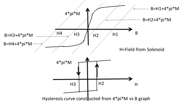
Figure 1.

In figure 1 above,  the hysteresis curve of ## 4 \pi M ## vs. ## H ## is generated from the graph of ## 4 \pi M ## vs. ## B ## which is the characteristic magnetization curve for a typical ferromagnetic material.

Conclusion:

The reader should now have a better understanding of the role of the magnetic surface currents in maintaining the magnetization in a permanent magnet and in generating the magnetic fields both inside and outside the permanent magnet.