Rindler Motion in Special Relativity: Hyperbolic Trajectories

Introduction: Why Rindler Motion?

When students learn relativity, it’s usually taught using inertial (constant velocity) motion. There are lots of reasons for this, but mainly it’s because it’s the easiest kind of motion for deriving the results of relativity, and historically, thinking about inertial motion is what led to Einstein’s theory.  An unfortunate side-effect of the focus on inertial motion is that it often gives students the mistaken impression that Special Relativity only applies to inertial motion, and if you want to do something more complicated, you have to use General Relativity.

The second simplest type of motion to consider, which often is not covered in a student’s first course in relativity, is Rindler motion: the motion of a  rocket undergoing constant (proper) acceleration. Rindler motion is simple enough that it is possible to calculate many quantities of interest without using much more than simple calculus (the big benefit of inertial motion is that you hardly need calculus at all; it’s just algebra). But Rindler motion is a very good introduction to so many concepts that are important in understanding General Relativity:

• The apparent “gravity” comes from using noninertial coordinates.
• “Gravitational” time dilation
• Event horizons and coordinate singularities
• Coordinate system “patches” that only cover part of spacetime

The analogs between Rindler motion and gravity are many, and extend even to the frontiers of physics: there is an analog of black hole Hawking radiation, called Unruh radiation, associated with Rindler motion. (Although the derivation of Unruh radiation is beyond my abilities—maybe someone smarter than me can make an Insight post about it).

I plan to derive some of the basic facts about Rindler motion, using simple mathematics as much as possible.

What is Rindler Motion?

So what exactly is Rindler motion? Roughly, we can say that it is the motion of an object such as a rocket undergoing constant acceleration. However, in Special Relativity, unlike Newtonian physics, acceleration is a frame-dependent quantity, so we have to be a little more careful in saying what we mean by constant acceleration. So here’s my definition:

We will say that a rocket is undergoing Rindler motion if it is traveling along a single spatial direction such that at every moment, the acceleration of the rocket is always some constant, as measured in a frame in which the rocket is momentarily at rest.

That’s kind of a mouthful, so let’s unpack it a little. A rocket will have a particular velocity, $v$ and a particular acceleration, $a$. These are frame-dependent quantities. But if you pick a frame in which $v = 0$, then $a = g$, where $g$ is some constant.

What we would like to know is what Rindler motion looks like from the original launch frame. The rocket launches from Earth at time $t = 0$, and we’d like to know what its location is at some later value of $t$. It’s a little bit tricky to figure this out because velocity and acceleration transform in sort of complicated ways from frame to frame. However, there is a trick that makes computing things a snap, almost a matter of algebra, which is to use Lorentz invariants.

Spacetime Vectors and Lorentz Invariants

In the first course on Special Relativity, students are usually introduced to the Lorentz transformation. If you have two inertial coordinate systems (for simplicity, I’m only going to talk about one spatial dimension) $(x,t)$ and $(x’, t’)$ and they are lined up so that the events with coordinates $x’ = 0$ in the primed system correspond to the line $x=vt$ in the unprimed system, (so that the spatial origin of the primed system is moving at speed $v$ relative to the unprimed system) then the two systems will be related by:

• Equation 1: $x’ = \gamma (x – v t)$
• Equation 2: $t’ = \gamma (t – \frac{vx}{c^2})$

where $\gamma = \frac{1}{\sqrt{1-\frac{v^2}{c^2}}}$

What’s actually more useful than these transformation rules are the Lorentz invariants, which are quantities that have the same value in any inertial coordinate system. The beauty of invariants is that you can compute them using whatever coordinate system is most convenient.

I’m going to change to a more uniform way of doing the transformations, by considering not $x$ and $t$, but two coordinates I will call $x^1 \equiv x$ and $x^0 \equiv c t$. I multiply the time coordinate by $c$ to make the components both have units of length. In terms of these coordinates, the transformations become:

• Equation 3: $(x^1)’ = \gamma (x^1 – \frac{v}{c} x^0)$
• Equation 4: $(x^0)’ = \gamma (x^0 – \frac{v}{c} x^1)$

I’m going to use the phrase spacetime vector to mean any pair of quantities $V^0$ and $V^1$ that transforms in this way under a change of frames. (It’s usually called a 4-vector, for the 4 dimensions of spacetime, but that doesn’t make sense in my case, since I’m only dealing with 2 dimensions). Here’s the power of spacetime vectors: Let $V$ be one spacetime vector with coordinates $(V^0, V^1)$. Let $U$ be another spacetime vector with coordinates $(U^0, U^1)$. While the 4 components of $U$ and $V$ change from one frame to another, there is a combination that remains invariant:

$U \cdot V \equiv (U^0) (V^0) – (U^1)(V^1)$

Clearly, we have that the pair $x^0, x^1$ are components of a spacetime vector. What other spacetime vectors are there?

As I said earlier, velocity and acceleration transform in sort of complicated ways when you change frames. So they are not spacetime vectors. However, we can get related quantities that are spacetime vectors.

Getting back to our rocket, let $\tau$ be the time on a clock onboard the rocket. Pick an inertial coordinate system, $x,t$ and let $x(\tau)$ be the value of $x$ for the rocket when the rocket’s clock shows time $\tau$. Let $t(\tau)$ similarly be the time coordinate at which the rocket’s clock shows time $\tau$. Then for each value of $\tau$, the following pairs are all spacetime vectors:

• “Position”: $X \equiv (x(\tau), c t(\tau))$
• “Proper velocity”: $V \equiv \frac{dX}{d\tau} \equiv (\frac{dx}{d\tau}, \frac{d (c t)}{d\tau})$
• “Proper acceleration”: $A \equiv \frac{dV}{d\tau} \equiv (\frac{d^2 x}{d\tau^2}, \frac{d^2 (ct)}{d \tau^2}$

These spacetime vectors are the rocket’s position, proper velocity, proper acceleration. These are a little inverted from what people are used to. Usually, people describe changes in terms of time, but this way of looking at it describes the time coordinate as a function of proper time (also known as clock time, or elapsed time) $\tau$.

(Note: the spacetime “position” $X$ is only a spacetime vector in Special Relativity.  In the curved spacetime that is considered for General Relativity, it is no longer a vector, because it’s not possible to add positions that you add vectors. However, the proper velocity and proper acceleration continue to be spacetime vectors.)

We can use these spacetime vectors to completely solve the problem of Rindler motion.

Invariants for Rindler Motion

Now, getting back to Rindler motion, but now armed with the tool of spacetime vectors and invariants, we can restate the facts about Rindler motion.

After the rocket has already launched and has been accelerating for some time, it will have some velocity $v$ and some acceleration $a$. We pick an inertial coordinate system in which $v=0$. What’s nice about this frame is that the distinction between $\tau$ the time on the rocket’s clock and $t$ the coordinate time disappears. If the rocket is at rest, or traveling nonrelativistically, its clock will advance at the rate of one clock second for each coordinate time second that passes. That means that, at least initially, $\frac{dt}{d\tau} = 1$. So we can approximately replace derivatives with respect to $\tau$ by derivatives with respect to $t$.

In this coordinate system, we have the following facts about our spacetime vectors $V$ and $A$:

$V^1 \equiv \frac{dX^1}{d\tau} = \frac{dx}{d\tau} \approx \frac{dx}{dt} = 0$

The rocket is initially at rest in this frame, so $x$ isn’t changing, so its derivative is zero.

$V^0 \equiv \frac{dX^0}{d\tau} = \frac{d (ct)}{d\tau} = c \frac{d t}{d\tau} = c$

For proper acceleration,

$A^0 = \frac{d V^0}{d\tau} = 0$

$A^1 = \frac{dV^1}{d\tau} = \frac{d^2 X^1}{d\tau^2} \approx \frac{d^2 x}{dt^2} = g$

We can form the following invariants:

• Equation 5: $V \cdot V \equiv (V^0)^2 – (V^1)^2 = c^2$
• Equation 6: $A \cdot A \equiv (A^0)^2 – (A^1)^2 = -g^2$
• Equation 7: $V \cdot A \equiv V^0 A^0 – V^1 A^1 = 0$

Even though we derived these invariants in the special frame in which the rocket is momentarily at rest, they have the same value in every frame. With a tiny bit of algebra, and the assumption that all four quantities are positive, we can easily derive the following facts, true in every frame:

• Equation 8: $A^1 = \frac{g}{c} V^0$
• Equation 9: $A^0 = \frac{g}{c} V^1$

Remembering that by definition, $A^1 = \frac{dV^1}{d\tau}$ and $A^0 = \frac{dV^0}{d\tau}$, we can rewrite these facts completely in terms of $V$

• Equation 10: $\frac{dV^1}{d\tau} = \frac{g}{c} V^0$
• Equation 11: $\frac{dV^0}{d\tau} = \frac{g}{c} V^1$

We also know, by definition, that $\frac{dX^1}{d\tau} = V^1$ and $\frac{dX^0}{d\tau} = V^0$. So we discover a fact relating $X$ to $V$:

• Equation 12: $\frac{dX^1}{d\tau} = V^1 = \frac{c}{g} \frac{dV^0}{d\tau}$
• Equation 13: $\frac{dX^0}{d\tau} = V^0 = \frac{c}{g} \frac{dV^1}{d\tau}$

X-V Equations

We can integrate both sides of equations 12 and 13 with respect to $\tau$ to get:

• Equation 14: $X^1(\tau) – X^1(0) = \frac{c}{g}(V^0(\tau) -V^0(0))$
• Equation 15: $X^0(\tau) – X^0(0) = \frac{c}{g}(V^1(\tau) -V^1(0))$

In these equations, $X^1(\tau), X^0(\tau), V^1(\tau), V^0(\tau)$ are the spacetime position and proper velocity of the rocket when its clock shows time $\tau$. $X^1(0), X^0(0), V^1(0), V^0(0)$ are the initial values of position and proper velocity when the rocket’s clock shows time 0 (when the rocket first launches).

X-V Equations in Launch Frame

Equations 14 and 15 are valid in any inertial coordinate system whatsoever. But they become simpler in the original launch frame of the rocket. In this frame, we have:

• When $t=0$, $\tau = 0$ (the clock rocket is initially set to the time in the launch frame). Since $X^0 = c t$, we also have $X^0(0) = 0$.
• When $t=0$, $V^1 = 0$ (initially, the rocket is at rest, so its spatial velocity is 0)
• When $t=0$, $V^0 = c$ (We have the invariant $(V^0)^2 – (V^1)^2 = c^2$)

With these facts, we have (original launch frame only):

• Equation 16: $X^1(\tau) – X^1(0) = \frac{c}{g}(V^0(\tau) -c)$
• Equation 17: $X^0(\tau)  = \frac{c}{g}V^1(\tau)$

Since $(V^0)^2 – (V^1)^2 = c^2$, we can write:

Equation 18: $(X^1(\tau) – X^1(0) + \frac{c^2}{g})^2 – (X^0(\tau))^2 = \frac{c^4}{g^2}$

Returning to our more traditional coordinates #x# and #t#, we have:

Equation 19: $(x-x(0) + \frac{c^2}{g})^2 – c^2 t^2 = \frac{c^4}{g^2}$

or

Equation 20: $x = x(0) – \frac{c^2}{g} + \sqrt{ c^2 t^2 + \frac{c^4}{g^2}}$

A special choice of initial conditions sets $x(0) = \frac{c^2}{g}$, so the trajectory becomes even simpler:

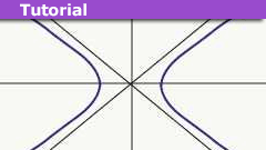
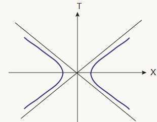
$x = \sqrt{ c^2 t^2 + \frac{c^4}{g^2}}$

This shows the dependence of spatial location $x$ as a function of coordinate time $t$ in the launch frame of the rocket. This functional dependence is hyperbolic motion, drawn in the upper-right-hand quadrant of the first figure of this article. As you can see, when $t \rightarrow \infty$, the motion approaches the diagonal line $x= ct$.

Coming up: Rindler Coordinates