A Black Hole Problem From Greg Egan’s “Incandescence”

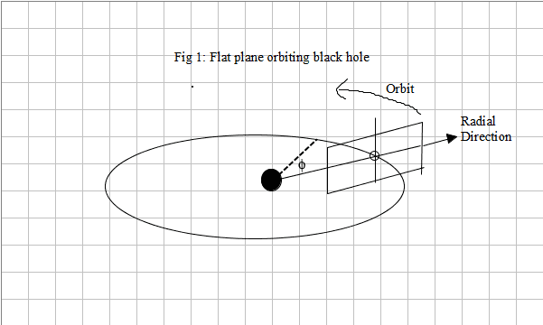
The following problem was inspired by reading Greg Egan’s “Incadescence”.  Consider a body, orbiting a Schwarzschild black hole and tide locked to it, as in figure 1 below.  The body itself has negligible mass, but due to the tidal gravity around the black hole, an observer on the body will feel “weight”.  The basic problem is to draw a map of this weight.

What do we mean by weight?  We first need a notion of a rigid body.  Then we can equate the weight of an observer on the body to the negative of their proper acceleration.  For instance, if we imagine an observer on an elevator which is accelerating upwards (“Einstein’s elevator”), their weight will point downwards, opposite to the direction of their acceleration, but equal in magnitude.

We will imagine the size of the body to be small, much smaller than the circumference of the orbit.  The body is three-dimensional, but it’s difficult – and unnecessary – to draw a three-dimensional map of the weight.  We will instead draw a map of the weight on a two-dimensional plane, as shown in figure 1.  This map shows the weight on a surface of constant $\phi$.  The value of $\phi$ is irrelevant, the symmetry of the problem means the map won’t change if we change the value of $\phi$.  Therefore we can omit the direction represented by a change in $\phi$ from our map.

Note that because the body is tide locked, the plane in figure 1 rotates as the body orbits.

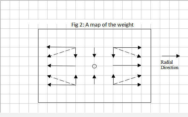
Figure 2 shows a sketch of the map in figure 1 seen “head-on”.  We’ve labeled one direction on this diagram the “radial” direction.  We’ll call the other direction on this diagram, perpendicular to the radial direction, the normal direction.

Onto the calculations.   We will do two calculations, one of which is more straightforwards, the other which is a little harder, but gives more insight.

We start by defining the line element of our metric (in geometric units) which is the Schwarzschild metric.

$$g =  -\left( 1 – \frac {2\,M}{r} \right) dt^2  + \frac{dr^2}{1-\frac {2\,M}{r}}  +r^2\, d\theta^2 + r^2 \, \sin^2 \theta \, d\phi^2$$

Now we need to define our rigid body.  The notion of a rigid body can be mathematically represented by a congruence of timelike worldlines, each worldline of the congruence representing the path through space-time of a point on the body.  The congruence we are interested in is $\phi = \omega t$.   To proceed further, we find the four-velocity u of a point on the congruence.  The components of u are:

$$u^0 = \frac{dt}{d\tau} = \frac{1}{\sqrt{1-\frac{2M}{r}-\omega^2 \, r^2 \, \sin^2 \theta}} \quad u^1=\frac{dr}{d\tau}=0 \quad u^2=\frac{d\theta}{d\tau}=0 \quad u^3=\frac{d\phi}{d\tau} =\frac{\omega}{\sqrt{ 1-\frac{2M}{r}-\omega^2 \, r^2 \, \sin^2 \theta}}$$

Using the idea from differential geometry that vectors are directional derivatives, we can re-write this in a different but equivalent notation as:

$$u =u^0\,\frac{\partial}{\partial t}+u^1\,\frac{\partial}{\partial r} + u^2\,\frac{\partial}{\partial \theta}+u^3\,\frac{\partial}{\partial \phi} =  \frac{\frac{\partial}{\partial t} + \omega \, \frac{\partial}{\partial \phi}} {\sqrt{1-\frac{2M}{r}-\omega^2 \, r^2 \, \sin^2 \theta}}$$

The “weight”, as we mentioned previously, is mathematically represented by the negative of the four-acceleration.  To compute the four-acceleration from the four-velocity we write $a = u^b \nabla_b u^a$.  Here $\nabla_b$ is the covariant derivative operator, the result $\nabla_b u^a$ is a rank two tensor which gives us the rate of change of u in any direction we specify.  Multiplying this rank two tensor by $u^b$ and contracting gives us the rate of change of u “in u direction”, i.e. the four-acceleration.

$$a = \left( \frac{\left( {\frac {M}{r^2}}-{r}{\omega}^{2}\sin^2  \theta \right)  \left( 1-{\frac {2M}{r}} \right)}{1 – \frac{2M}{r} – r^2 \, \omega^2 \, \sin^2 \theta }\right) \frac{\partial}{\partial r} -\left( \frac { \omega^2 \, \sin \theta \cos \theta} {1 -\frac{2M}{r} – r^2 \, \omega^2 \, \sin^2 \theta } \right) \frac{\partial}{\partial\theta} $$

The orbital plane is given by $\theta = \frac{\pi}{2}$.  For a circular orbit, the r-coordinate value will be constant,  we will call this constant $r_0$.  Knowing that at $r_0$ the 4-accleration on the orbital plane is zero,  we can solve for $\omega = \sqrt{ \frac{M}{r_0^3}}.$

Since we assume that the body is small, we can greatly simplify the above expression by expanding it in terms of the first order.  We first note that to the first order, we can write $\sin \theta \approx 1$ and $\cos \theta \approx – \left(\theta – \frac{\pi}{2} \right)$ at $\theta = \frac{\pi}{2}$.  We can then expand the expression for the radial component via a taylor series around $r = r_0$.  The resulting linear approximation gives us the two components of a:

$$ a = a_r \frac{\partial}{\partial r} + a_\theta \frac{\partial}{\partial \theta} \quad a_r \approx – \frac{3M}{r_0^3} \left( \frac{1 – \frac{2M}{r_0} } {1 – \frac{3M}{r_0} } \right) \left( r – r_0 \right) \quad a_\theta \approx \frac{M}{r_0^3} \left( \frac{1}{1 – \frac{3M}{r_0} } \right) \left( \theta – \frac{\pi}{2} \right)$$

We can write the displacement as

$$d = \left(r – r_0\right) \frac{\partial}{\partial r} + \left(\theta – \frac{\pi}{2} \right) \frac{\partial}{\partial \theta}$$

Note that we are computing the displacement in the tangent space (since we are representing it as a vector), rather than on the manifold itself.

Direct physical interpretation of our results, such as the physical reading of a scale measuring the weight of a unit mass, is hindered by the fact that we’ve expressed the results in terms of basis vectors that are not of unit length.  The length of a vector is given by $\sqrt{|g_{ij} \, p^i \, p^j|}$, and if we calculate the length of the vector $\partial / \partial \theta$, we see that it’s length is not 1 but r.  The vector $\partial / \partial r$ does not have a unit length either.

At a later point, we will change our basis to one where the basis vectors do have unit length, an orthonormal basis.  At this point, however, we’ll simply note that if we express displacements in terms of multiples of a vector of arbitrary length, and we express accelerations in multiples of the same vector, the ratio of acceleration to displacement does not depend on the length of the arbitrary vector.

In the radial direction, we can calculate this ratio (the ratio of the radial weight to the radial displacement) as:

$$k_r = \,-\frac{3M}{r_0^3} \left( \frac{1 – \frac{2M}{r_0} } {1 – \frac{3M}{r_0} } \right)$$

In the normal direction, we calculate the ratio of the normal weight to the normal displacement as:

$$k_\theta=\frac{M}{r_0^3} \left( \frac{1}{1 – \frac{3M}{r_0} } \right)$$

The radial weight points away from the center while the normal weight points towards the center.  Finally, the ratio of the radial weight to the normal weight for a unit displacement , $k_r / k_\theta$, is equal to $-3 + 6M/r_0$.  This matches (modulo sign conventions) the result in “Incadescence”.  While the book is fictional, the math is thoughtful, deep, and accurate, though informally presented.

We also note that both $k_r$ and $k_\theta$ increase without bound as r approaches $3M$.  This seems sensible because $r=3M$ is the photon sphere, where the proper time to complete an orbit approach zero.  Of course, circular orbits wouldn’t be stable this close to the black hole, the radius of the minimum stable orbit is at $r=6M$.

Additionally, we note that for large r, the ratio $k_r / k_\theta$ becomes -3:1, the same as in the Newtonian limit.

We will now proceed to get the same result, using a different, less direct procedure.  This approach, while less direct, provides more physical insight.  Conceptually it’s much closer to the approach that Egan uses in his hard science fiction novel.

In the preceding section, we simply calculated the weight directly.  In the following section, we will divide the weight into two distinct source categories.  We will calculate each category separately, and add them together at the end.   One part of the weight is caused by geodesic deviation, the other part is caused by the rotation of our reference plane.  The effects of the rotation is basically to add a centrifugal force component of the weight in two of the three directions – the radial direction, and the un-mapped direction.  No weight due to rotation is added to the normal direction, as that direction is the axis of rotation.

The part of the weight that’s due to geodesic deviation can be calculated by the geodesic deviation equation.

$$a^a = R^a{}_{bcd} \, u^b \, d^c \, u^d $$

If we let

$$E^a{}_c= R^a{}_{bcd} \, u^b \, u^d$$

we can write $a^a = E^a{}_c d^c$, which gives us the acceleration as a linear map from displacement.  Thus this tensor is a linear map from displacement to the geodesic part of the weight.  These values of the components of E are directly comparable to the factors $k_r$ and $k_\theta$ that we calculated previously, except that they do not include the contribution of the rotation to the weight.

We use the same congruence of worldlines we used previously, defined by the same 4-velocity field u.  R is the Riemann tensor, d is a separation vector (from the center of the object).  a is  (modulo the sign issue) the non-rotational part of the weight, and E has already been described.

We will begin our computation by defining a frame of 4 vectors that are of unit length and orthogonal to each other, an orthonormal basis frame, for a shell observer, an observer with constant Schwarzschild coordinates.

$$\vec{e’}_0 = \frac{\frac{\partial}{\partial t}}{ \sqrt{1-\frac{2M}{r}}} \quad \vec{e’}_1= \left( \sqrt{1-\frac{2M}{r}} \right) \frac{\partial} {\partial r}  \quad \vec{e’}_2 = \frac{ \frac{\partial}{\partial \theta} }{r} \quad \vec{e’}_3=\frac{ \frac{\partial}{\partial \phi} }{r \, \sin \theta}$$

The mathematical requirement for a vector q to be of unit length is that $g_{ij}\, q^i\, q^j$ equals one for space-like vectors, and -1 for time-like vectors.  The mathematical requirement for two vectors p and q to be orthogonal is that $g_{ij}\, p^i \, q^j = 0$.  By performing these calculations, we can check our results.

An orbiting observer will have a different set of orthonormal basis vectors than our shell observer.  We construct this frame by boosting the frame of a shell observer in the $\vec{e’}_4$ direction by a velocity $\beta$.  We let $\gamma = 1/\sqrt{1-\beta^2}$.  We’ll drop the prime symbol for our new frame.  With the appropriate values for $\gamma$ and $\beta$, this will be the orthonrmal frame of an orbiting observer.  We can express the new frame in terms of the old as:

$$\vec{e}_0 = \gamma \vec{e’}_0 + \beta \gamma \vec{e’}_3 \quad \vec{e}_1 = \vec{e’}_1 \quad \vec{e}_2 = \vec{e’}_2 \quad  \vec{e}_3 = \gamma \vec{e’}_3 + \beta \gamma \vec{e’}_0$$

Note that with the appropriate values of $\beta$ and $\gamma$ (which we will compute later), $\vec{e}_0$ is the same as our four-velocity u.

At this point, we can carry out the calculation to find our linear map $E^a{}_b$ in the unprimed orthonormal basis that represents the frame field of an orbiting observer.  By expressing our tensors in terms of orthonormal basis vectors, the components of the tensors will directly correspond to the measured weights, unlike the previous results that were written on a coordinate basis.  The calculation of $E^a{}_b$ would be painfully long to carry out by hand, and the Riemann tensor would also be very long to write out, so we will simply give the result for $E^a{}_b$ from a computer calculation.  Most tensor analysis packages give the tensor components directly in any desired frame, though it is possible to break the computation into two parts, the first part being to find the tensor components on a coordinate basis, the second part being to convert the values of the components from a coordinate basis to an orthonormal basis via the tensor transformation rules.

Our frame vectors are $\left[ \vec{e}_0, \vec{e}_1, \vec{e}_2, \vec{e}_3 \right]$.   The duals of these vectors will be represented by $[\vec{\omega}^0, \vec{\omega}^1, \vec{\omega}^2, \vec{\omega}^3]$.   The use of a vector arrow symbol over the dual vectors is slightly non-standard, but aids in avoiding confusion between the dual vectors and the angular frequency $\omega$,  which uses the same base symbol.  Using this basis, we can write:

$$E = -\,\frac{2M}{r^3} \left( \frac{ 1+\frac{\beta^2}{2}} {1-\beta^2 } \right) \, \vec{e}_1 \vec{\omega}^1 +\frac{M } {r^3 }  \left( \frac{1+2 \beta^2 } {1 – \beta^2 }  \right) \, \vec{e}_2 \vec{\omega}^2 + \frac{M } {r^3 }\, \vec{e}_3 \vec{\omega}^3 $$

Now we find the values for $\beta$ and $\gamma$ that represents the velocity of an orbiting observer relative to a co-located shell observer.  Utilizing our previous result for the four-velocity, u, namely:

$$u = \frac{\frac{\partial}{\partial t} + \omega \, \frac{\partial}{\partial \phi}} {\sqrt{1-\frac{2M}{r}-\omega^2 \, r^2 \, \sin^2 \theta}}$$

We set $\theta = \pi/2$.

Next we set $\omega=0$ to get the 4-velocity of a stationary shell observer, and $\omega=\sqrt{\frac{M}{r^3}}$  to get the 4-velocity of our orbiting observer.

Taking the dot product of this pair of four-vectors gives the same result for relative velocity  that it would in special relativity, namely $-\gamma$.  Hence we can use the value of the dot product to find the needed values for $\gamma$ and $\beta$.

$$\gamma = \sqrt{ \frac{1 – \frac{2M}{r} } {1 – \frac{3M}{r} } } \quad \beta = \sqrt{\frac{\frac{M}{r} } {1-\frac{2M}{r} } }$$

We can substitute these values into our expressions for E to get the three components of the weight/displacement ratio:

$$\left[E^1{}_1 \quad E^2{}_2 \quad E^3{}_3\right] = \left[ -\frac{2M}{r^3} \left(  \frac{1 – \frac{3M}{2r} } {1 – \frac{3M}{r} }\right) \quad \frac{M}{r^3} \left( \frac{1}{1- \frac{3M}{r}} \right) \quad \frac{M}{r^3} \right] $$

We now want to account for the effects of the rotation of the frame.  We know that the centrifugal “weight” will have a magnitude of $\omega^2 \Delta r$, $\Delta r$ being a displacement not to be confused with r.  The ratio of the centrifugal weight to the displacement will just be $\omega^2$.  We already know that $\omega^2  = M/r^3$ from our previous analysis.  With the sign conventions we have been using, this contribution will be negative.  We can thus write the following adjustment factors for the rotational contribution to our weight/displacement ratio.

$$\left[ -\frac{M}{r^3} \quad 0 \quad -\frac{M}{r^3} \right]$$

Summing the geodesic and centrifugal contributions to the weight/displacement ratio, we get:

$$\left[ -\frac{3M}{r^3} \left(  \frac{1 – \frac{2M}{r} } {1 – \frac{3M}{r} } \right) \quad  \frac{M}{r^3} \left( \frac{1}{1- \frac{3M}{r}} \right) \quad 0\right]$$

We note that the weight ratio vanishes in the $\vec{e}_3$ direction, as expected, and the weight ratios in the other two directions match our previous calculations.