
Why the Quantum | A Response to Wheeler’s 1986 Paper
Wheeler’s opening statement in his 1986 paper, “How Come the Quantum?” holds as true today as it did then [1]
The necessity of the quantum in the construction of existence: out of what deeper requirement does it arise? Behind it all is surely an idea so simple, so beautiful, so compelling that when — in a decade, a century, or a millennium — we grasp it, we will all say to each other, how could it have been otherwise? How could we have been so stupid for so long?
In this Insight, I will answer Wheeler’s question per its counterpart in quantum information theory (QIT), “How come the Tsirelson bound?” Let me start by explaining the Tsirelson bound and its relationship to the Bell inequality, then it will be obvious what that has to do with Wheeler’s question, “How Come the Quantum?” The answer (the Tsirelson bound is a consequence of conservation per no preferred reference frame (NPRF)) may surprise you with its apparent simplicity, but that simplicity belies a profound mystery, as we will see.
The Tsirelson bound is the spread in the Clauser-Horne-Shimony-Holt (CHSH) quantity
\begin{equation}\langle a,b \rangle + \langle a,b^\prime \rangle + \langle a^\prime,b \rangle – \langle a^\prime,b^\prime \rangle \label{CHSH1}\end{equation}
created by quantum correlations. Here, we consider a pair of entangled particles (or “quantum systems” or “quantum exchanges of momentum”). Alice makes measurements on one of the two particles with her measuring device set to ##a## or ##a^\prime## while Bob makes measurements on the other of the two particles with his measuring device set to ##b## or ##b^\prime##. There are two possible outcomes for either Bob or Alice in either of their two possible settings given by ##i## and ##j##. For measurements at ##a## and ##b## we have for the average of Alice’s results multiplied by Bob’s results on a trial-by-trial basis
\begin{equation}\langle a,b \rangle = \sum (i \cdot j) \cdot P(i,j \mid a,b) \label{average}\end{equation}
That’s a bit vague, so let me supply some actual physics. The two entangled states I will use are those which uniquely give rise to the Tsirelson bound [2-4] , i.e., the spin singlet state and the ‘Mermin photon state’ [5]. The spin singlet state is ##\frac{1}{\sqrt{2}} \left(\mid ud \rangle – \mid du \rangle \right)## where ##u##/##d## means the outcome is displaced upwards/downwards relative to the north-south pole alignment of the Stern-Gerlach (SG) magnets (Figure 1).
 Figure 1. A Stern-Gerlach (SG) spin measurement showing the two possible outcomes, up and down, represented numerically by +1 and -1, respectively. Figure 42-16 on page 1315 of Physics for Scientists and Engineers with Modern Physics, 9th ed, by Raymond A. Serway and John W. Jewett, Jr.
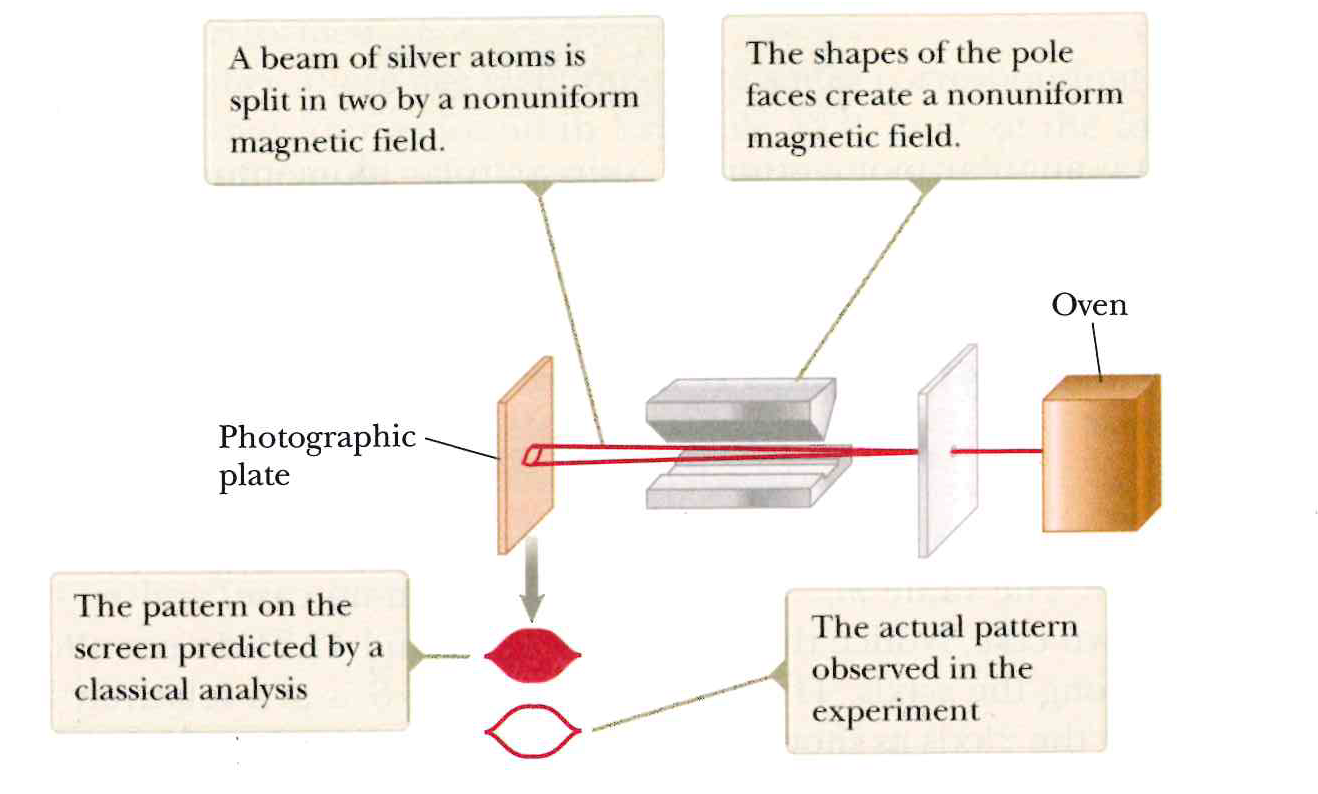 Figure 1. A Stern-Gerlach (SG) spin measurement showing the two possible outcomes, up and down, represented numerically by +1 and -1, respectively. Figure 42-16 on page 1315 of Physics for Scientists and Engineers with Modern Physics, 9th ed, by Raymond A. Serway and John W. Jewett, Jr.
This state obtains due to conservation of angular momentum at the source as represented by momentum exchange in the spatial plane P orthogonal to the source collimation (“up or down” transverse). This state might be produced by the dissociation of a spin-zero diatomic molecule [6] or the decay of a neutral pi meson into an electron-positron pair [7], processes which conserve spin angular momentum. For more information about the spin singlet state and the spin triplet states, see this Insight.
The Mermin state for photons is ##\frac{1}{\sqrt{2}} \left(\mid VV \rangle + \mid HH \rangle \right)## where ##V## means the there is an outcome (photon detection) behind one of the coaligned polarizers and ##H## means there is no outcome behind one of the co-aligned polarizers. This state obtains due to conservation of angular momentum at the source as represented by momentum exchange along the source collimation (“yes” or “no” longitudinal). Dehlinger and Mitchell created this state by laser inducing spontaneous parametric downconversion in beta barium borate crystals [8], a process that conserves spin angular momentum as represented by the polarization of the emitted photons. At this point we will focus the discussion on the spin single state for total anti-correlation, since everything said of that state can be easily transferred to the Mermin photon state.
Let us investigate what Alice and Bob discover about these entangled states in the various contexts of their measurements (Figure 2). Alice’s detector responds up and down with equal frequency regardless of the orientation ##\alpha## of her SG magnet. This is in agreement with the relativity principle, aka “no preferred reference frame” (NPRF), where different SG magnet orientations relative to the source constitute different “reference frames” in quantum mechanics just as different velocities relative to the source constitute different “reference frames” in special relativity (see this Insight).

Figure 2. Alice and Bob making spin measurements in the xz plane on a pair of spin-entangled particles with their Stern-Gerlach (SG) magnets and detectors.
Bob observes the same regarding his SG magnet orientation ##\beta##. Thus, the source is rotationally invariant in the spatial plane P orthogonal to the source collimation. When Bob and Alice compare their outcomes, they find that their outcomes are perfectly anti-correlated (##ud## and ##du## with equal frequency) when ##\alpha – \beta = \theta = 0## (Figure 3). This is consistent with conservation of angular momentum per classical mechanics between the pair of detection events (again, this fact defines the state). The degree of that anti-correlation diminishes as ##\theta \rightarrow \frac{\pi}{2}## until it is equal to the degree of correlation (##uu## and ##dd##) when their SG magnets are at right angles to each other. In other words, whenever the SG magnets are orthogonal to each other anti-correlated and correlated outcomes occur with equal frequency, i.e., conservation of angular momentum in one direction is independent of the angular momentum changes in any orthogonal direction. Thus, we wouldn’t expect to see more correlation or more anti-correlation based on conservation of angular momentum for transverse results in the plane P when the SG magnets are orthogonal to each other. As we continue to increase the angle ##\theta## beyond ##\frac{\pi}{2}## the anti-correlations continue to diminish until we have totally correlated outcomes when the SG magnets are anti-aligned. This is also consistent with conservation of angular momentum, since the totally correlated results when the SG magnets are anti-aligned represent momentum exchanges in opposite directions in the plane P just as when the SG magnets are aligned, it is now simply the case that what Alice calls up, Bob calls down and vice-versa.
The counterpart for the Mermin photon state is simply that angular momentum conservation is evidenced by ##VV## or ##HH## outcomes for coaligned polarizers. When the polarizers are at right angles you have only ##VH## and ##HV## outcomes, which is still totally consistent with conservation of angular momentum as ‘not ##H##’ implies ##V## and vice-versa [8]. In other words, a polarizer does not have a ‘north-south’ distinction (longitudinal rather than transverse momentum exchange). In particular, having rotated either or both polarizers by ##\pi## one should obtain precisely ##VV## or ##HH## outcomes again.
Nothing is particularly mysterious about the entangled states for electron spin or photon polarization described here so far because we have been thinking as if conservation of angular momentum holds for each experimental trial, as in classical mechanics. Truth is, since Alice and Bob can only measure +1 or -1 (quantum exchange of momentum per NPRF), we can only get conservation of angular momentum in any particular trial when their SG magnets/polarizers are co-aligned. And, we cannot use classical probability theory to account for the conservation of angular momentum on average.
In particular, the probability that Alice and Bob will measure ##uu## or ##dd## at angles ##\alpha## and ##\beta## for the spin singlet state is
\begin{equation}P_{uu} = P_{dd} = \frac{1}{2} \mbox{sin}^2 \left(\frac{\alpha – \beta}{2}\right) \label{probabilityuu}\end{equation}
And, the probability that Alice and Bob will measure ##ud## or ##du## at angles ##\alpha## and ##\beta## for the spin singlet state is
\begin{equation}P_{ud} = P_{du} = \frac{1}{2} \mbox{cos}^2 \left(\frac{\alpha – \beta}{2}\right) \label{probabilityud}\end{equation}
Using these in Eq. (\ref{average}) where the outcomes are +1 (##u##) and -1 (##d##) gives Eq. (\ref{CHSH1}) of
\begin{equation}-\cos(a – b) -\cos(a – b^\prime) -\cos(a^\prime – b) +\cos(a^\prime – b^\prime) \label{CHSHspin}\end{equation}
Choosing ##a = \pi/4##, ##a^\prime = -\pi/4##, ##b = 0##, and ##b^\prime = \pi/2## minimizes Eq. (\ref{CHSHspin}) at ##-2\sqrt{2}## (the Tsirelson bound).
Likewise, for the Mermin photon state we have
\begin{equation}P_{VV} = P_{HH} = \frac{1}{2} \mbox{cos}^2 \left(\alpha – \beta \right) \label{probabilityVV}\end{equation}
and
\begin{equation}P_{VH} = P_{HV} = \frac{1}{2} \mbox{sin}^2 \left(\alpha – \beta \right) \label{probabilityVH}\end{equation}
Using these in Eq. (\ref{average}) where the outcomes are +1 (##V##) and -1 (##H##) gives Eq. (\ref{CHSH1}) of
\begin{equation}\cos2(a – b) +\cos2(a – b^\prime) +\cos2(a^\prime – b) -\cos2(a^\prime – b^\prime) \label{CHSHmermin}\end{equation}
Using ##a = \pi/8##, ##a^\prime = -\pi/8##, ##b = 0##, and ##b^\prime = \pi/4## maximizes Eq. (\ref{CHSHmermin}) at ##2\sqrt{2}## (the Tsirelson bound). So, we have two mysteries.
First, as explained by Mermin [5], suppose you restrict Alice and Bob’s measurement angles ##\alpha## and ##\beta## to three possibilities, setting 1 is ##0^o##, setting two is ##120^o##, and setting three is ##-120^o##. Eq. (\ref{probabilityud}) says the probability of getting opposite results is 1 when ##\alpha = \beta## (1/2 ##ud## and 1/2 ##du##) and 1/4 otherwise (1/8 ##ud## and 1/8 ##du##). Now, if the source emits particles with definite properties that account for their outcomes in the three possible measurement settings, and we have to get total anti-correlation for like settings, then the particles’ so-called “instruction sets” must be opposite for each of the three settings. For example, suppose we have 1(##u##)2(##u##)3(##d##) for Alice and 1(##d##)2(##d##)3(##u##) for Bob. That guarantees the total anti-correlation for like settings, i.e., 11 gives ##ud##, 22 gives ##ud##, and 33 gives ##du##. And, for unlike settings we get anti-correlation in two combinations, i.e., 12 gives ##ud## and 21 gives ##ud##. In fact, for any instruction set with two ##u## and one ##d## we get anti-correlation for unlike settings in two of the six possible unlike combinations (12,13,21,23,31,32). The only other way to make a pair of instruction sets is to have one with all ##u## and the other with all ##d##. In that case, we get anti-correlation for all six unlike combinations. That means the instruction sets necessary to guarantee anti-correlation for like settings lead to an overall anti-correlation greater than 2/6 for unlike settings, which is greater than the quantum probability for anti-correlation in unlike settings of 1/4. This is Mermin’s version of the Bell inequality [9] (fraction of anti-correlated outcomes for unlike settings must be greater than 2/6) and the manner by which it is violated by quantum correlations (1/4 is less than 2/6). Thus, instruction sets (“counterfactual definiteness”) assumed by classical probability theory cannot account for quantum correlations in this case.
The counterpart to this for the CHSH quantity is that classical correlations give a range of -2 to 2 for the CHSH quantity (“CHSH-Bell inequality”). And, as we saw above, the Tsirelson bound violates the CHSH-Bell inequality. Experiments show that the quantum results can be achieved (violating the Bell inequality), ruling out an explanation of these correlated momentum exchanges via instruction sets per classical probability theory.
The second mystery is that even in cases where we don’t violate the Bell inequality, e.g., ##a = b = 0## and ##a^\prime = b^\prime = \pi/2## which give a CHSH value of 0, we still have conservation of angular momentum. Why is that mysterious? Well, it’s not when the SG magnets are co-aligned, since in those cases we always get a +1 outcome and a -1 outcome for a total of zero. But, in trials where ##\alpha – \beta = \theta## does not equal zero, we need either Alice or Bob, at minimum, to measure something less than 1 to conserve angular momentum. For example, if Alice measures +1, then Bob must measure ##-\cos{\theta}## to conserve angular momentum for that trial. But, again, Alice and Bob only measure +1 or -1 (quantum exchange of momentum per NPRF, which uniquely distinguishes the quantum joint distribution from its classical counterpart [10]), so that can’t happen (Figure 4). What does happen? We conserve angular momentum on average in those trials.
It is easy to see how this follows by starting with total angular momentum of zero for binary (quantum) outcomes +1 and -1 (I am suppressing the factor of ##\hbar/2## and I’m referring to the spin singlet state here [11], Figure 3).
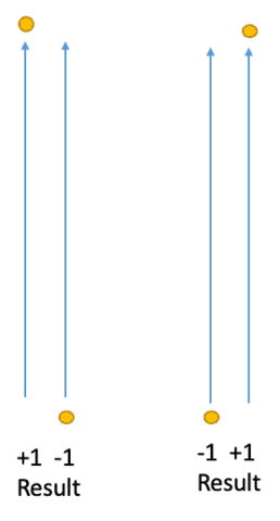
Figure 3. Outcomes (yellow dots) in the same reference frame, i.e., outcomes for the same measurement (blue arrows represent SG magnet orientations), for the spin singlet state explicitly conserve angular momentum.
Alice and Bob both measure +1 and -1 results with equal frequency for any SG magnet angle (NPRF) and when their angles are equal they obtain different outcomes giving total angular momentum of zero. The case (a) result is not difficult to understand via conservation of angular momentum, because Alice and Bob’s measured values of spin angular momentum cancel directly when ##\alpha = \beta##, that defines the spin singlet state. But, when Bob’s SG magnet is rotated by ##\alpha – \beta = \theta## relative to Alice’s, the situation is not as clear (Figure 6).
In classical physics, one would say the projection of the angular momentum vector of Alice’s particle ##\vec{S}_A = +1\hat{a}## along ##\hat{b}## is ##\vec{S}_A\cdot\hat{b} = +\cos{(\theta)}## where again ##\theta## is the angle between the unit vectors ##\hat{a}## and ##\hat{b}## (Figure 2). From Alice’s perspective, had Bob measured at the same angle, i.e., ##\beta = \alpha##, he would have found the angular momentum vector of his particle was ##\vec{S}_B = -1\hat{a}##, so that ##\vec{S}_A + \vec{S}_B = \vec{S}_{Total} = 0##. Since he did not measure the angular momentum of his particle at the same angle, he should have obtained a fraction of the length of ##\vec{S}_B##, i.e., ##\vec{S}_B\cdot\hat{b} = -1\hat{a}\cdot\hat{b} = -\cos{(\theta)}## (Figure 4).
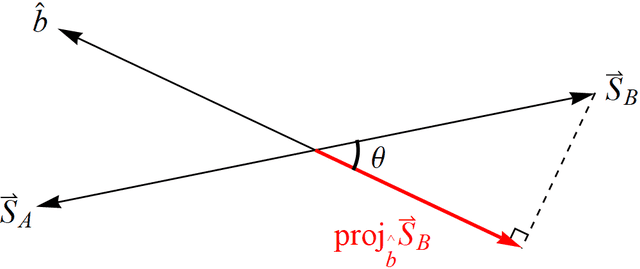
Figure 4. The projection of the angular momentum of Bob’s particle ##\vec{S}_B## along his measurement direction ##\hat{b}##. This does not happen with spin angular momentum due to NPRF.
Of course, Bob only ever obtains +1 or -1 per NPRF, so Bob’s outcomes can only average the required ##-\cos{(\theta)}##. Thus, NPRF dictates
\begin{align*}
P_{uu} + P_{ud} & = \frac {1}{2} \\
P_{ud} + P_{dd} & = \frac {1}{2},
\end{align*}
These equations now allow us to uniquely solve for the joint probabilities
\begin{equation}
P_{uu} = P_{dd} = \frac{1}{2} \mbox{sin}^2 \left(\frac{\theta}{2} \right) \label{QMjointLike}
\end{equation}
and
\begin{equation}
P_{ud} = P_{du} = \frac{1}{2} \mbox{cos}^2 \left(\frac{\theta}{2} \right) \label{QMjointUnlike}
\end{equation}
\begin{equation}
\overline{BA-} = 2P_{du}(+1) + 2P_{dd}(-1) = \cos (\theta) \label{BA-}
\end{equation}
Using Eqs. (\ref{BA+}) and (\ref{BA-}) in Eq. (\ref{consCorrel}) we obtain
\begin{equation}
\langle \alpha,\beta \rangle = \frac{1}{2}(+1)_A(-\mbox{cos} \left(\theta\right)) + \frac{1}{2}(-1)_A(\mbox{cos} \left(\theta\right)) = -\mbox{cos} \left(\theta\right) \label{consCorrel2}
\end{equation}
which is precisely the correlation function for a spin singlet state found using the joint probabilities per quantum mechanics. To see that we simply use Eqs. (\ref{probabilityuu}) and (\ref{probabilityud}) in Eq. (\ref{average}) to get
\begin{equation}
\begin{split}
\langle \alpha,\beta \rangle = &(+1)(-1)\frac{1}{2} \mbox{cos}^2 \left(\frac{\alpha – \beta}{2}\right) + (-1)(+1)\frac{1}{2} \mbox{cos}^2 \left(\frac{\alpha – \beta}{2}\right) +\\ &(+1)(+1)\frac{1}{2} \mbox{sin}^2 \left(\frac{\alpha – \beta}{2}\right) + (-1)(-1)\frac{1}{2} \mbox{sin}^2 \left(\frac{\alpha – \beta}{2}\right) \\ &= -\mbox{cos} \left(\alpha – \beta \right) = -\mbox{cos} \left(\theta \right)
\end{split}
\label{correl}\end{equation}
Thus, “average-only” conservation maps beautifully to our classical expectation (Figures 6 & 7). Since the angle between SG magnets ##\theta## is twice the angle between Hilbert space measurement bases, this result easily generalizes to conservation per NPRF of whatever the measurement outcomes represent when unlike outcomes entail conservation in the symmetry plane [15] (see this Insight on the Bell spin states). However, again, none of the formalism of quantum mechanics is used in obtaining Eq. (\ref{consCorrel2}) or our quantum state Eqs. (\ref{QMjointLike}) & (\ref{QMjointUnlike}). In deriving the quantum correlation function and quantum state in this fashion, we assumed only NPRF.For the Mermin photon state, conservation of angular momentum is established by ##V## (designated by +1) and ##H## (designated by -1) results through a polarizer. When the polarizers are co-aligned Alice and Bob get the same results, half pass and half no pass. Thus, conservation of angular momentum is established by the intensity of the electromagnetic radiation applied to binary outcomes for various polarizer orientations. As with spin angular momentum, this is classical thinking applied to binary outcomes per conservation of angular momentum. Again, grouping Alice’s results into +1 and -1 outcomes we see that she would expect to find ##[\mbox{cos}^2\theta – \mbox{sin}^2\theta]## at ##\theta## for her +1 results and ##[\mbox{sin}^2\theta – \mbox{cos}^2\theta]## for her -1 results. Since Bob measures the same thing as Alice for conservation of angular momentum, those are Bob’s averages when his polarizer deviates from Alice’s by ##\theta##. Therefore, the correlation of results for conservation of angular momentum is given by
\begin{equation}\langle \alpha,\beta \rangle =\frac{(+1_A)(\mbox{cos}^2\theta – \mbox{sin}^2\theta)}{2} + \frac{(-1_A)(\mbox{sin}^2\theta – \mbox{cos}^2\theta)}{2} = \cos{2\theta} \label{merminconserve}\end{equation}
which is precisely the correlation given by quantum mechanics.As before, we need to find ##P_{VV}##, ##P_{HH}##, ##P_{VH}##, and ##P_{HV}## so we need four independent conditions. Normalization and ##P_{VH} = P_{HV}## are the same as for the spin case. The correlation function
\begin{equation}
\begin{split}
\langle \alpha,\beta \rangle = &(+1)_A(+1)_BP_{VV} + (+1)_A(-1)_BP_{VH} + \\&(-1)_A(+1)_BP_{HV} + (-1)_A(-1)_BP_{HH}\label{correlFn2}
\end{split}
\end{equation}
along with our conservation principle represented by Eq. (\ref{merminconserve}) give
\begin{equation}
P_{VV} – P_{VH} = -\frac{1}{2}(\mbox{sin}^2\theta – \mbox{cos}^2\theta)
\end{equation}
and
\begin{equation}
P_{HV} – P_{HH} = \frac{1}{2}(\mbox{sin}^2\theta – \mbox{cos}^2\theta)
\end{equation}
Solving these four equations for ##P_{VV}##, ##P_{HH}##, ##P_{VH}##, and ##P_{HV}## gives precisely Eqs. (\ref{probabilityVV}) & (\ref{probabilityVH}).Notice that since the angle between polarizers ##\alpha – \beta## equals the angle between Hilbert space measurement bases, this result immediately generalizes to conservation per NPRF of whatever the outcomes represent when like outcomes entail conservation in the symmetry plane [15] (again, see this Insight on the Bell spin states).Since the quantum correlations violate the Bell inequality to the Tsirelson bound and satisfy conservation per NPRF while the classical correlations do not violate the Bell inequality, the classical correlations do not satisfy conservation per NPRF. Experiments of course tell us that Nature obeys the quantum correlations and therefore the conservation per NPRF.
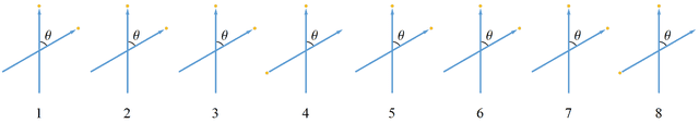
Figure 5. A spatiotemporal ensemble of 8 experimental trials for the Bell spin states showing Bob’s outcomes corresponding to Alice‘s ##+1## outcomes when ##\theta = 60^\circ##. Angular momentum is not conserved in any given trial, because there are two different measurements being made, i.e., outcomes are in two different reference frames, but it is conserved on average for all 8 trials (six up outcomes and two down outcomes average to ##\cos{60^\circ}=\frac{1}{2}##). It is impossible for angular momentum to be conserved explicitly in each trial since the measurement outcomes are binary (quantum) with values of ##+1## (up) or ##-1## (down) per no preferred reference frame. The conservation principle at work here assumes Alice and Bob’s measured values of angular momentum are not mere components of some hidden angular momentum with variable magnitude. That is, the measured values of angular momentum are the angular momenta contributing to this conservation.
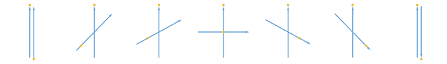
Figure 6. For the spin singlet state (S = 0). Reading from left to right, as Bob rotates his SG magnets relative to Alice’s SG magnets for her +1 outcome, the average value of his outcome varies from –1 (totally down, arrow bottom) to 0 to +1 (totally up, arrow tip). This obtains per conservation of angular momentum on average in accord with no preferred reference frame. Bob can say exactly the same about Alice’s outcomes as she rotates her SG magnets relative to his SG magnets for his +1 outcome. That is, their outcomes can only satisfy conservation of angular momentum on average, because they only measure +1/-1, never a fractional result. Thus, just as with the light postulate of special relativity, we see that no preferred reference frame leads to counterintuitive results (see this Insight).
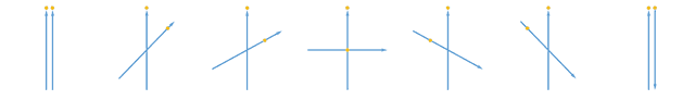
Figure 7. The situation is similar for the spin triplet states where outcomes agree for the same measurement in the plane containing the conserved angular momentum vector (S = 1). Reading from left to right, as Bob rotates his SG magnets relative to Alice’s SG magnets for her +1 outcome, the average value of his outcome varies from +1 (totally up, arrow tip) to 0 to –1 (totally down, arrow bottom). This obtains per conservation of angular momentum on average in the plane containing the S = 1 spin angular momentum in accord with no preferred reference frame. See this Insight for details.
So, while conservation per NPRF sounds like a very reasonable constraint on the distribution of quantum exchange of momentum (+1 or -1, no fractions), we still do not have any causal mechanism to explain the outcomes of any particular trial when the SG magnets/polarizers are not co-aligned (Figure 4). And, as I showed above, we cannot use instruction sets per classical probability theory to account for the Tsirelson bound needed to explain the conservation of angular momentum on average. Thus, while we have a very reasonable constraint on the distribution of entangled quantum exchanges (conservation of angular momentum), that constraint has no compelling dynamical counterpart, i.e., no consensus causal mechanism to explain the outcome of any particular trial when the SG magnets/polarizers are not co-aligned and no counterfactual definiteness to explain why conservation of angular momentum is conserved on average. What we have is a “principle” account of entanglement and the Tsirelson bound (see this Insight). I will return to this point after showing how so-called “superquantum correlations” fail to satisfy this constraint as well.
There are QIT correlations that not only violate the Bell inequality, but also violate the Tsirelson bound. Since these correlations violate the Tsirelson bound, they are called “superquantum correlations.” The reason QIT considers these correlations reasonable (no known reason to reject their possibility) is because they do not violate superluminal communication, i.e., the joint probabilities don’t violate the no-signaling condition
\begin{equation}\begin{split}P(A \mid a\phantom{\prime},b\phantom{\prime}) &= P(A \mid a\phantom{\prime}, b^\prime)\\
P(A \mid a^\prime,b\phantom{\prime}) &= P(A \mid a^\prime, b^\prime)\\
P(B \mid a\phantom{\prime},b\phantom{\prime}) &= P(B \mid a^\prime, b\phantom{\prime})\\
P(B \mid a\phantom{\prime},b^\prime) &= P(B \mid a^\prime, b^\prime )\end{split}\label{nosig}\end{equation}
This means Alice and Bob measure the same outcomes regardless of each other’s settings. If this wasn’t true, Alice and Bob would notice changes in the pattern of their outcomes as the other changed their measurement settings. Since the measurements for each trial can be spacelike separated that would entail superluminal communication.
The Popescu-Rohrlich (PR) joint probabilities
\begin{equation}\begin{split}&P(1,1 \mid a,b) = P(-1,-1 \mid a, b)=\frac{1}{2}\\
&P(1,1 \mid a,b^\prime) = P(-1,-1 \mid a, b^\prime)=\frac{1}{2}\\
&P(1,1 \mid a^\prime,b) = P(-1,-1 \mid a^\prime, b)=\frac{1}{2}\\
&P(1,-1 \mid a^\prime,b^\prime) = P(-1,1 \mid a^\prime, b^\prime)=\frac{1}{2} \end{split}\label{PRcorr}\end{equation}
produce a value of 4 for Eq. (\ref{CHSH1}), the largest of any no-signaling possibilities. Thus, the QIT counterpart to Wheeler’s question, “How Come the Quantum?” is “Why the Tsirelson bound?” [12-14]. In other words, is there any compelling principle that rules out superquantum correlations as conservation of angular momentum ruled out classical correlations? Let us look at Eq. (\ref{PRcorr}) in the context of our spin singlet and Mermin photon states. Again, we will focus the discussion on the spin singlet state and allude to the obvious manner by which the analysis carries over to the Mermin photon state.
The last PR joint probability certainly makes sense if ##a^\prime = b^\prime##, i.e., the total anti-correlation implying conservation of angular momentum, so let us start there. The third PR joint probability makes sense for ##b = \pi + b^\prime##, where we have conservation of angular momentum with Bob having flipped his coordinate directions. Likewise, then, the second PR joint probability makes sense for ##a = \pi + a^\prime##, where we have conservation of angular momentum with Alice having flipped her coordinate directions. All of this is perfectly self consistent with conservation of angular momentum as we described above, since ##a^\prime## and ##b^\prime## are arbitrary per rotational invariance in the plane P. But now, the first PR joint probability is totally at odds with conservation of angular momentum. Both Alice and Bob simply flip their coordinate directions, so we should be right back to the fourth PR joint probability with ##a^\prime \rightarrow a## and ##b^\prime \rightarrow b##. Instead, the first PR joint probability says that we have total correlation (maximal violation of conservation of angular momentum) rather than total anti-correlation per conservation of angular momentum, which violates every other observation. In other words, the set of PR observations violates conservation of angular momentum in a maximal sense. To obtain the corresponding argument for angular momentum conservation per the correlated outcomes of the Mermin photon state, simply start with the first PR joint probability and show the last PR joint probability maximally violates angular momentum conservation.
To find the degree to which superquantum correlations violate our constraint, replace the first PR joint probability with
\begin{equation}\begin{split}&p(1,1 \mid a,b) = C \\
&p(-1,-1 \mid a, b) = D \\
&p(1,-1 \mid a,b) = E \\
&p(-1,1 \mid a, b) = F \\ \end{split} \label{PRcorrMod}\end{equation}
The no-signaling condition Eq. (\ref{nosig}) in conjunction with the second and third PR joint probabilities gives ##C = D## and ##E = F##. That in conjunction with normalization ##C + D + E + F =1## and P(anti-correlation) + P(correlation) = 1 means total anti-correlation (##E = F = 1/2##, ##C = D = 0##) is the conservation of angular momentum per the quantum case while total correlation (##E = F = 0##, ##C = D = 1/2##) is the max violation of conservation of angular momentum per the PR case. To get the corresponding result for the Mermin photon state, simply replace the last PR joint probability in analogous fashion, again with ##\theta = \pi##. In that case, the PR joint probabilities violate conservation of angular momentum with total anti-correlation while the Mermin photon state satisfies conservation of angular momentum with total correlation. Thus, we have a spectrum of superquantum correlations all violating conservation of angular momentum.
So, we see explicitly in this result how quantum mechanics conforms statistically to a conservation principle without need of a ‘causal influence’ or hidden variables acting on a trial-by-trial basis to account for that conservation. That is the essence of a “principle theory.” Indeed, the kinematic structure (Minkowski spacetime) of special relativity and the kinematic structure (qubit Hilbert space) of quantum mechanics both follow from NPRF, so we now know that quantum mechanics is on par with special relativity as a principle theory (again, see this Insight).
Therefore, my answer to QIT’s version of Wheeler’s question is
The Tsirelson bound obtains because of conservation per no preferred reference frame.
Whether or not you consider this apparently simple 4-dimensional (4D) constraint (conservation per NPRF [16,17,18]) to dispel the mystery of entanglement and answer Wheeler’s question depends on whether or not you can accept the fundamentality of a principle explanation via patterns in both space and time (see this Insight). While we have a compelling 4D constraint (who would argue with conservation per NPRF?) for our adynamical explanation, we do not have a compelling dynamical counterpart. That is, we do not have a consensus, causal mechanism to explain outcomes on a trial-by-trial basis when the SG magnets/polarizers are not co-aligned, and we cannot use counterfactual definiteness per classical probability theory to account for the fact that we conserve angular momentum on average. So, perhaps we do not need new physics to rise to Wilczek’s challenge [19].
To me, ascending from the ant’s-eye view to the God’s-eye view of physical reality is the most profound challenge for fundamental physics in the next 100 years.
[Note: “God’s-eye view” simply means the blockworld, block universe, “all-at-once”, or 4D view like that of Minkowski spacetime, there is no religious connotation.] Since special relativity already supports that view, perhaps we should accept that adynamical explanation is fundamental to dynamical explanation, so that not all adynamical explanations have dynamical counterparts [20]. In that case, “we will all say to each other, how could it have been otherwise? How could we have been so stupid for so long?” [1]
References
- Wheeler, J.A.: How Come the Quantum?, New Techniques and Ideas in Quantum Measurement Theory 480(1), 304–316 (1986).
- Cirel’son, B.S.: Quantum Generalizations of Bell’s Inequality, Letters in Mathematical Physics 4, 93–100 (1980).
- Landau, L.J.: On the violation of Bell’s inequality in quantum theory, Physics Letters A 120(2), 54–56 (1987).
- Khalfin, L.A., and Tsirelson, B.S.: Quantum/Classical Correspondence in the Light of Bell’s Inequalities, Foundations of Physics 22(7), 879–948 (1992).
- Mermin, N.D.: Bringing home the atomic world: Quantum mysteries for anybody, American Journal of Physics 49(10), 940–943 (1981).
- Bohm, D.: Quantum Theory, Prentice-Hall, New Jersey (1952).
- La Rosa, A.: Introduction to Quantum Mechanics, Chapter 12
- Dehlinger, D., and Mitchell, M.W.: Entangled photons, nonlocality, and Bell inequalities in the undergraduate laboratory, American Journal of Physics 70(9), 903–910 (2002).
- Bell, J.: On the Einstein-Podolsky-Rosen paradox, Physics 1, 195–200 (1964).
- Garg, A., and Mermin, N.D.: Bell Inequalities with a Range of Violation that Does Not Diminish as the Spin Becomes Arbitrarily Large, Physical Review Letters 49(13), 901–904 (1982).
- Unnikrishnan, C.S.: Correlation functions, Bell’s inequalities and the fundamental conservation laws, Europhysics Letters 69, 489–495 (2005).
- Bub, J.: Bananaworld: Quantum Mechanics for Primates, Oxford University Press, Oxford, UK (2016).
- Bub, J.: Why the Quantum?, Studies in History and Philosophy of Modern Physics 35B, 241–266 (2004).
- Bub, J.: Why the Tsirelson bound?, in The Probable and the Improbable: The Meaning and Role of Probability in Physics, eds. Meir Hemmo and Yemima Ben-Menahem, Springer, Dordrecht, 167–185 (2012).
- Weinberg, S.: The Trouble with Quantum Mechanics (2017).
- Stuckey, W.M., Silberstein, M., McDevitt, T., and Kohler, I: Why the Tsirelson Bound? Bub’s Question and Fuchs’ Desideratum, Entropy 21(7), 692 (2019).
- Stuckey, W.M., Silberstein, M., McDevitt, T., and Le, T.D.: Answering Mermin’s challenge with conservation per no preferred reference frame, Scientific Reports 10, 15771 (2020).
- Silberstein, M., Stuckey, W.M., and McDevitt, T.: Beyond Causal Explanation: Einstein’s Principle Not Reichenbach’s, Entropy 23(1), 114 (2021).
- Wilczek, F.: Physics in 100 Years, Physics Today 69(4), 32–39 (2016).
- Silberstein, M., Stuckey, W.M., and McDevitt, T.: Beyond the Dynamical Universe: Unifying Block Universe Physics and Time as Experienced, Oxford University Press, Oxford, UK (2018).
PhD in general relativity (1987), researching foundations of physics since 1994. Coauthor of “Beyond the Dynamical Universe” (Oxford UP, 2018).


Leave a Reply
Want to join the discussion?Feel free to contribute!