How to Model a Magnet Falling Through a Solenoid

Introduction

Modeling a magnet realistically is a task best done numerically.  Even the simplified model of two separated disks with uniform surface magnetization $\pm~\sigma_M$ involves elliptic integrals simplifying assumptions. As a model, the point dipole may be unrealistic to some but the math is tractable and accessible.  The usefulness of the point dipole model in electrodynamics is analogous to that of the point mass in kinematics and dynamics.  It brings forth the salient features and serves as a starting point for more involved treatments.  Indeed, analyses of the falling magnet found in the literature rely on modifications of the point dipole equations with an eye toward bringing their predictions into better agreement with experiments.

The goal of this article is to gather in one place what can be said about a magnet dipole falling through a solenoid.  A second article, now in preparation, has the same goal but for a point magnetic dipole falling through a solid conducting pipe.

The motional emf

The inverse Lorentz transformation equations for the components of the electric and magnetic fields are $$\begin{align}& \mathbf{E}_{\parallel}=\mathbf{E’}_{\parallel}~;~~\mathbf{B}_{\parallel}=\mathbf{B’}_{\parallel}\nonumber \\& \mathbf{E}_{\perp} =\gamma\left(\mathbf{E’}_{\perp} -\mathbf{v}\times\mathbf{B’}\right)~;~~\mathbf{B}_{\perp}=\gamma\left(\mathbf{B’}_{\perp}-\frac{1}{c^2}\mathbf{v}\times\mathbf{E’}\right).\nonumber \end{align}$$

Consider a magnetic point dipole $\mathbf{m}=m~\hat z$ falling with velocity $\mathbf{v}=v~\hat z$.  Taking “down” as positive  and for ordinary magnet velocities ($\gamma \approx 1$), we write in cylindrical coordinates,$$\mathbf{E}_{\perp}=-\mathbf{v}\times \mathbf{B’}=-\mathbf{v}\times \mathbf{B}=-v~\hat z\times\left(B_{\rho}~\hat {\rho}+B_z~\hat {z}\right)=-vB_{\rho}~\hat {\theta}.$$The line integral $\int_a^b \mathbf{E}_{\perp}\cdot d\mathbf{l}$ is the motional emf between points $a$ and $b$.

The relativistic treatment might be a bit too much, but it helps get the signs right.  Anyway, from here on we will discontinue the use of primes to denote coordinates in the moving frame. Instead, we will use primes for source coordinates and no primes for coordinates of points of interest. Integrals will be taken over primed coordinates.

A single ring

At point of interest $\mathbf{r}(\rho ,z)$ when the dipole is at $\mathbf{r’}(\rho’,z’)$ the dipolar field is $$\mathbf{B}=\frac{\mu_0}{4\pi} \left[ \frac{ \left(3 \mathbf{m}\cdot (\mathbf{r}-\mathbf{r}’))(\mathbf{r}-\mathbf{r}’)-|\mathbf{r}-\mathbf{r}’|^2 \mathbf{m}\right)}{|\mathbf{r}-\mathbf{r}’|^5}  -\frac{\mathbf{m}}{ |\mathbf{r}-\mathbf{r}’|^3}  \right].$$We place the dipole on the $z$-axis and orient it so that $\mathbf{m}=m~\hat z$. At  $\rho=a$, the radial component of the magnetic field is $$B_{\rho}=\frac{3\mu_0ma}{4\pi}  \frac{ z-z’} {\left[a^2+(z-z’)^2\right]^{5/2}}.$$

The motional emf in a coaxial single ring of radius $a$ at $z’$ is $$\begin{align}\text{emf}_{\text{ring}}=\int \mathbf{E}_{\perp}\cdot d\mathbf{l}=-vB_{\rho}(2\pi a) = -\frac{3\mu_0ma^2}{2}  \frac{ (z-z’)~v} {\left[a^2+(z-z’)^2\right]^{5/2}}.\end{align}$$Note that the ring could be an intangible loop, not necessarily conducting, and the emf around it would still exist.  If, however, the ring is a conducting loop, there will be an induced current in it.  A plot of the spatial dependence of the emf is shown in Figure 1 below. We note that when the dipole is farther than about 4 radii from the ring’s center, the emf is below 1% of its peak value.

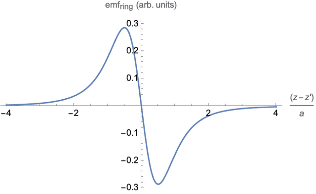
Figure 1. Single ring emf as a function of dipole position.

As the dipole falls in free space,  a wave of motional emf with the waveform shown in Figure 1 is traveling with velocity $v(t)$ down an intangible tube consisting of  loops of radius $a.$  In the next section, we will explore what to expect when a conducting finite solenoid of radius $a$ occupies part of that space.

From ring to solenoid

We imagine the solenoid as a stack of  $N$ turns. The beginning of the $k$th turn is the end of the $(k-1)$th and the end of the $k$th turn is the beginning of the $(k+1)$th.  Thus, the turns are a collection of rings connected in series.  We are seeking an expression for the emf across the free ends of a solenoid of $N$ turns, radius $a$, and length $L$. It will be an integral of  $\text{emf}(z)$ over the length of the solenoid.

The number of rings in a stack of height $dz’$ is $dn=\dfrac{N}{L}dz’$. Integrating over the length, $$\begin{align}\text{emf}(z)=\frac{N}{L}\int_{\frac{-L}{2}}^{\frac{L}{2}}\text{emf}_{\text{ring}}dz’=\frac{\mu _0 N m a^2}{2 L} \left\{ \frac{v}{\left[a^2+\left(z-\frac{L}{2}\right)^2\right]^{3/2}}-\frac{v}{\left[a^2+\left(z+\frac{L}{2}\right)^2\right]^{3/2}}\right\}.\end{align}$$

We assume that the dipole has mass and is in free fall.  If the solenoid ends are open, there will be an emf across them but no current.  Even when a voltmeter is connected to measure the emf, the current through it is expected to be negligible . In either case, eddy current braking is negligible and we will ignore it together with air resistance.  Under these circumstances, the standard kinematic equations under constant acceleration apply.  Taking the origin at the midpoint of the solenoid, we write an expression for the position of the dipole. We assume that it starts from rest at height $h$ above the top of the solenoid ($z_0=-h-\frac{L}{2}$.) Substituting $$z=(-h-\frac{L}{2}+\frac{1}{2}g~t^2)~\text{ and }~v=g~t$$ in equation (2), we obtain the emf across the solenoid as a function of time. $$\begin{align}\text{emf}(t)=\frac{\mu _0 N m a^2}{2 L} \left\{ \frac{g~t}{\left[a^2+\left(-h-L+\frac{1}{2}g~t^2\right)^2\right]^{3/2}}-\frac{g~t}{\left[a^2+\left(-h+\frac{1}{2}g~t^2\right)^2\right]^{3/2}}\right\}\end{align}$$

The emf profile

Figure 2 below is a plot of emf(t) vs $t$ without the overall multiplicative constant.  For the plot, we used  $g=980$ for the acceleration, $a=1$ for the radius, $h=6a$ for the release height above the top and $L=10 a$ for the length. Thus,  if the units for the radius $a$ are centimeters, the numbers on the abscissa will be seconds.  The solid vertical grid lines mark the times when the dipole is at the top, midpoint, and bottom of the solenoid. The pairs of red dashed lines mark the times when the dipole is within one solenoid diameter ($\pm~2a$) from the top (left) and the bottom (right).

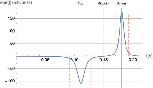
Figure 2. Solenoid emf as a function of time.

Alternatively, we can obtain an expression for the emf as a function of position $z$ by substituting $v=\sqrt{2g[z-(-h-\frac{L}{2})]}$ in equation (2) to get $$\begin{align}\text{emf}(z)=\frac{\mu _0 N m a^2}{2 L} \left\{\frac{\sqrt{2 g \left(z+h+\frac{L}{2}\right)}}{\left[a^2+\left(z-\frac{L}{2}\right)^2\right]^{3/2}}-\frac{\sqrt{2 g \left(z+h+\frac{L}{2}\right)}}{\left[a^2+\left(z+\frac{L}{2}\right)^2\right]^{3/2}}\right\}.\end{align}$$A plot of the emf($z$) vs. $z$ is not shown because it is identical to the one in figure 2 except for the labeling of the abscissa. Both plots feature extrema, one negative and one positive, with a region between when/where the emf is near zero. This is qualitatively consistent with Faraday’s law. The magnetic flux changes most rapidly when the dipole is near the ends and hardly at all when it is near the middle of the solenoid.

Term corrections

Examination of figure 2 reveals that the extrema occur when the dipole is near the ends of the solenoid. At $z=+L/2$ the first term in equation (4) has a maximum while the second term is small; the reverse is true at $z=-L/2$. An exact determination of the extrema would involve solving $\frac{d}{dz}\text{emf}(z)=0$, a daunting task. Considering, however, that the true extrema are very close to $z=\pm \frac{L}{2}$, it is expedient to do series expansions of equation (4) about $z=\pm \frac{L}{2}$ to second-order and find corrections to the zeroth-order terms.  Here, we summarize the results and relegate some of the details to the Appendix.

The fractional corrections to the position and value of the minimum are $$\frac{\delta z}{(-L/2)}=-5.5\times 10^{-3}~;~~\frac{\delta(\text{emf})}{\text{emf}(-L/2)}=1.1\times 10^{-3}.$$The corresponding numbers for the maximum are $$\frac{\delta z}{(+L/2)}=2.1\times 10^{-3}~;~~\frac{\delta( \text{emf})}{\text{emf}(L/2)}=1.6\times 10^{-4}.$$The numbers show that the corrections have a small effect on the zeroth order terms. Thus, we will ignore them and make the algebra easier.

A relation between amplitudes

We define as amplitudes the magnitudes of the extrema of $\text{emf}(t)$ (Figure 2). In the approximation that the extrema occur at $z=\pm ~\frac{1}{2}$,  equation (4) gives, the amplitudes $$\begin{align} & A_1=\left|\text{emf}(-L/2)\right|=\sqrt{2 g h}\left[\frac{1}{a^3}-\frac{1}{\left(a^2+L^2\right)^{3/2}}\right]\nonumber \\ &  A_2=\text{emf}(+L/2)|=\sqrt{2 g (h+L)}\left[\frac{1}{a^3}-\frac{1}{\left(a^2+L^2\right)^{3/2}}\right].\nonumber \end{align}$$

We write the difference between the two equations as $$\begin{align} &  A_2-A_1=\text{const.} \left(\sqrt{\frac{2 (h+L)}{g}}-\sqrt{\frac{2 h}{g}}\right) \nonumber \\ & \text{where  }\text{const.}=\frac{\mu _0 N m a^2}{2 g L}\left[\frac{1}{a^3}-\frac{1}{\left(a^2+L^2\right)^{3/2}}\right].\nonumber \end{align}$$We recognize the expression in parentheses multiplying the constant as the transit time $T$ of the dipole from one end of the solenoid to the other. This simplifies the equation even more to $$\begin{align}A_2-A_1=(\text{const.})\times T.\end{align}$$

It is easy to imagine an experimental protocol to test equation (5) with equipment that samples and records the emf across the solenoid as a function of time. However, one should ensure that starting heights $h$ are greater than the effective dipole range of 4 solenoid radii. This will minimize experimental uncertainties that become significant at small values of $h$. A PF thread posted by @billy_t here describes such an experiment. However, the analysis focused on the amplitudes themselves and not on their relation to the time of transit.

Summary

Modeling a magnet as a point dipole falling through a solenoid is sufficient to provide a sensible description of the shape and general features of the emf($t$) curve that is in agreement with what one would expect qualitatively.  The flux varies most rapidly when the dipole is entering and exiting the solenoid and least rapidly when it is near the solenoid’s middle. The amplitude of the right peak is greater than the left. This happens because its width is narrower since the dipole is moving faster, yet the area under the curve is the same. It is unlikely that a more realistic model of the magnet will result in a different interpretation of these features. A sophisticated model needs sophisticated data analysis to match it, perhaps one involving a point-by-point simulation of the entire curve.

Acknowledgments

I thank @billyT_ for posting the thread quoted above; it seeded this insight. Also, the participation of @haruspex and @Charles Link honed my thinking and is greatly appreciated.

Appendix

The work shown here was Mathematica-assisted.  In equation (4) we first drop $g$ and substitute reduced lengths $\lambda=L/a,~\eta=h/a$. Then expand the equation for small values of $\epsilon = z\pm \lambda/2$ to second order.  Each expansion yielded a quadratic expression $A\epsilon^2+B\epsilon+C.$  Setting the derivative equal to zero and solving for $\epsilon$ gives $\epsilon=\frac{-B}{2A}$.  Omitting the gory details, the corrections for the minimum on the left and the maximum on the right are:

$$\begin{align} & \epsilon_{\text{min}}  =\frac{2 \eta \left(\lambda ^2+1\right) \left[\left(\lambda ^2+1\right)^{5/2}-\left(6 \eta \lambda +\lambda ^2+1\right)\right]}{\left(12 \eta ^2+1\right) \left(\lambda ^2+1\right)^{7/2}+12 \eta ^2 \left(4 \lambda ^2-1\right)+12 \eta \lambda \left(\lambda ^2+1\right)-\left(\lambda ^2+1\right)^2}\nonumber \\ & \epsilon_{\text{max}}  =\frac{ 2 \left(\lambda ^2+1\right) (\eta +\lambda ) \left[6 \eta \lambda +\left(\lambda ^2+1\right)^{5/2}+5 \lambda ^2-1\right]}    {12 \eta ^2 \left(4 \lambda ^2-1\right)+12 \eta \lambda\left(7 \lambda ^2-3\right)  +\left(\lambda ^2+1\right) \left[12 \left(\lambda ^2+1\right)^{5/2} (\eta +\lambda )^2+1\right]+\left(35 \lambda ^4-26 \lambda ^2-1\right)}\nonumber \end{align}$$Figure 3 shows a detail of figure 2 in the vicinity of the maximum.  The vertical line is at the corrected value of $z/a$.  The zeroth order term of the expansion is to its left at $z/a=5.00$.

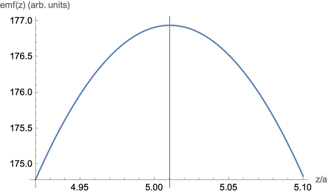
Figure 3. Detail of the correction to the zeroth order term.