How to Model a Magnet Falling Through a Conducting Pipe

Introduction

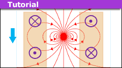
In an earlier article, we examined a magnet falling through a solenoid. We argued that the point dipole model can account for the basic features of the induced emf across the solenoid ends. Here, we extend the model to a magnet falling through a conducting pipe along its axis.

With the falling dipole moment oriented along the vertical $z$-axis, the electric field $E(\rho,z)$ is tangent to circles centered on the axis.  The induced emf around a closed loop of radius $\rho$ is $\text{emf}(z)=2\pi \rho~E(\rho,z)$. There is a similarity and a difference between a solenoid and a conducting pipe placed in that space.  The similarity is in their modeling as a stack of conducting rings. The difference is in the conceptual connection of the constituent rings.  In the solenoid, the rings are in series and the overall emf across them is of interest.  In the pipe, the rings are sort of in parallel and the total current through them is of interest. “Sort of” indicates that the emf, being position-dependent, is not the same from one ring to the next.

Nonetheless, Lenz’s law dictates that the induced currents will oppose the motion of the falling magnet.  In the segment beneath the dipole, they will be in repulsion while in the segment above the dipole they will be in attraction with the magnet.  We will add these forces to find the net electromagnetic force on the magnet. We will then solve Newton’s second law equation to obtain an expression suitable for elementary data analysis.

A single ring

We have seen that the motional emf in a coaxial single ring of radius $a$ located at $z’$ is $$\begin{align}\text{emf}_{\text{ring}}= -\frac{3\mu_0ma^2}{2}  \frac{ (z-z’)~v} {\left[a^2+(z-z’)^2\right]^{5/2}}.\end{align}$$Here, the positive $z$ axis is “down”.  The dipole with magnetic moment $\mathbf{m}=m~\hat{z}$ is on the axis at $z$.

Finding the current and its field

The current in the ring is $$\begin{align}I=\frac{\text{emf}}{R}= -\frac{3\mu_0ma^2}{2R}  \frac{ (z-z’)~v} {\left[a^2+(z-z’)^2\right]^{5/2}}\end{align}$$where $R$ is the ring’s resistance. The on-axis magnetic field generated by this current at the location of the dipole is $$\mathbf{B}_{\text{ring}}=\frac{\mu_0 a^2 I~\hat{z}}{\left[(a^2+(z-z’)^2\right]^{3/2}}.$$ We assume that the ring is beneath the dipole ($z-z'<0$) and that the dipole points in the positive $z$ direction.  By Lenz’s law, the field and the dipole moment must be antiparallel.

Finding the force

We will obtain the force on the dipole using energy considerations. The potential energy is $$U=-\mathbf{m}\cdot\mathbf{B}_{\text{ring}}=+m{B}_{\text{ring}}=\frac{\mu_0 m a^2 I}{\left[(a^2+(z-z’)^2\right]^{3/2}}$$and the force on the dipole is $$\mathbf{F}=-\mathbf{\nabla}U=-\mu_0 m a^2 I\frac{\partial}{\partial z}\left\{\frac{1}{\left[(a^2+(z-z’)^2\right]^{3/2}}\right\}~\hat z=\frac{3 \mu _0 a^2 I (z-z’)}{2 \left[a^2+(z-z’)^2\right]^{5/2}}~\hat z.$$With the current from equation (2) the magnetic force on the dipole is $$\begin{align}\mathbf{F}=-\frac{ 9 \mu _0^2 m^2 a^4 (z-z’) ^2 ~v ~\hat{z}}{4 R \left[a^2+(z-z’) ^2\right]^5}.\end{align}$$The force exerted by the ring on the dipole is negative (up) for all values of the dipole-loop separation $z-z’.$ A separate calculation (not shown) of the integral $\oint I d\mathbf{l} \times \mathbf{B}_{dip}$ confirms that the force exerted on the ring by the dipole is consistent with Newton’s third law and equation (3).

Figure 1 shows the dependence of the magnitude of the force on the dipole as a function of the reduced dipole-loop separation $\zeta=(z-z’)/a.$ The force is zero when the dipole passes through the center of the ring.  That’s because the current goes through zero before it reverses direction. However, the force also goes through zero at the center, yet it does not reverse direction and displays a characteristic two hump profile.  Also, the force is significant only inside a region of about $\pm$ 2 ring radii from the center.

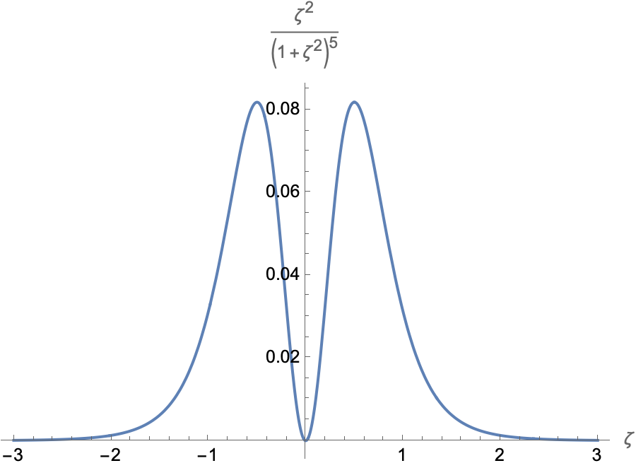
Figure 1. The spatial dependence of the force on the dipole exerted by a current loop as a function of the reduced distance between the two.

From ring to conducting pipe

We place the origin at the midpoint of a pipe of length $L$. The net force on the dipole is the vector sum of all ring contributions over the length of the pipe.  First, we convert equation (3) to a force element $d\mathbf{F}$.  We consider a ring of radius $\rho’$ and rectangular cross-sectional area $dA’ =dz’\times d\rho’$. The resistance of this ring is $$dR=\frac{2\pi \rho’}{\sigma~d\rho’~dz’}$$where $\sigma$ is the conductivity.  Then $$d\mathbf{F}=-\frac{ 9\sigma \mu _0^2 m^2 {\rho’}^3 (z-z’) ^2 ~v }{8\pi \left[{\rho’}^2+(z-z’) ^2\right]^5}~d\rho’~ dz’~\hat{z}$$

We define a force factor $\mathcal{F}(z)$ as the double integral without the constants, the velocity and the negative sign:

$$\begin{align}\mathcal{F}(z)\equiv\int_{-L/2}^{L/2}(z-z’)^2~dz’\int_{a}^{b}\frac{{\rho’}^3}{\left[{\rho’}^2+(z-z’) ^2\right]^5}~d\rho’.\end{align}$$ Built in it is the geometric information of the pipe: length $L$, inner diameter $a$ and outer diameter $b$.

The integrals

Assisted by Mathematica, we find the radial integral,

$$\int_a^b \frac{ {\rho’}^3 ~d\rho’}{\left[{\rho’}^2+(z-z’) ^2\right]^5}=\frac{4 a^2+(z-z’) ^2}{24 \left[a^2+(z-z’) ^2\right]^4}-\frac{4 b^2+(z-z’) ^2}{24 \left[b^2+(z-z’) ^2\right]^4}.$$

We will break up and compact the results of the axial integration over $z’$ in order to fit them on the screen.  We have,

$$ \begin{align}& \int_{-L/2}^{L/2}\frac{\left(z-z’)^2[4 a^2+(z-z’) ^2\right]}{24 \left[a^2+(z-z’) ^2\right]^4}dz’=\nonumber \\& \left .\frac{1}{384a^3}\left\{\frac{a (z-z’) \left[5 a^4-8 a^2 \left(z-z’\right)^2-5 (z-z’)^4\right]}{\left[a^2+\left(z-z’\right)^2\right]^3}-5 \tan ^{-1}\left(\frac{z-z’}{a}\right)\right\}
\right |_{z’=-L/2}^{z’=L/2}\nonumber \end{align}$$

and

$$ \begin{align}&- \int_{-L/2}^{L/2}\frac{\left(z-z’)^2[4 b^2+(z-z’) ^2\right]}{24 \left[b^2+(z-z’) ^2\right]^4}dz’=\nonumber \\& \left . -\frac{1}{384b^3}\left\{\frac{b (z-z’) \left[5 b^4-8 b^2 \left(z-z’\right)^2-5 (z-z’)^4\right]}{\left[b^2+\left(z-z’\right)^2\right]^3}-5 \tan ^{-1}\left(\frac{z-z’}{b}\right)\right\} \right |_{z’=-L/2}^{z’=L/2}\nonumber \end{align}$$

The sum of the evaluated terms above is the force factor $\mathcal{F}(z).$

The force factor

Figure 2 shows two plots for the force factor $\mathcal{F}(z)$ for two outer radii, $b=1.25a$ (blue line) and $b=2a$ (orange line). The pipe length was set at $L=100a$.  The plots indicate that the force factor rises fast, is flat, and rises higher for the thicker pipe.  We will deal with these features and what it all means in FAQ format.

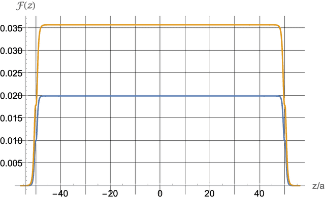
Figure 2. The force factor as a function of position for two values of the outer diameter, 1.25 a (blue) and 2.0 a (orange). The length of the pipe is 100 a.

How fast does it rise?

Since the effective range of the dipole is four inner radii, we would expect $\mathcal{F}(z)$ to change appreciably within that distance from the ends.  Figure 3 below shows a detail of Figure 2 and confirms this. The first vertical line is at the entry point at $z/a=-L/(2a)=-50.$ The second vertical line is at at $z/a=-L/(2a)+2=-48.$  It is where we consider the dipole to be “just fully inside” the pipe.   Clearly, the force factor is quite flat there. That’s pretty fast.

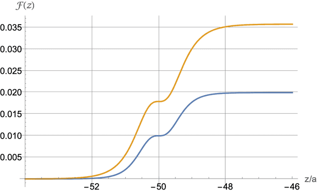
Figure 3. Detail of Figure 2 near the point of entry at -50.

The plateau at the point of entry can be understood by referring to the double-humped force shown in Figure 1.  Very near the point of entry the force due to the first infinitesimal ring and its near neighbors is small and decreasing, goes through zero, and then increases.  The total force stays flat until the dipole is far enough inside for the second hump to kick in.  Once fully inside there is a steady-state.  New rings ahead of the dipole come into range while old ones behind the dipole fade out of range.

Yes, but how flat is “flat”?

We take as a measure of flatness is the percent ratio $\mathcal{F}(-48)/\mathcal{F}(0)$.  It is the ratio of the value of the force factor at 2 ring radii in to the value in the middle.  For the pipe with $b=1.25a$ (blue line),  the ratio is 99.3%; for the pipe with $b=2~a$ it is 98.2%.  That’s pretty flat.

How does the wall thickness affect it?

We calculated the value at the midpoint $\mathcal{F}(0)$ as a function of the reduced outer radius $b/a$. Figure 4 below shows the resulting plot. It seems that beyond $b\approx 2a$, making the wall thicker produces diminishing returns. This makes sense. On one hand, increasing the wall thickness introduces more charge carriers in the space. On the other hand, the magnetic field that induces these currents becomes weaker with distance at a faster rate.

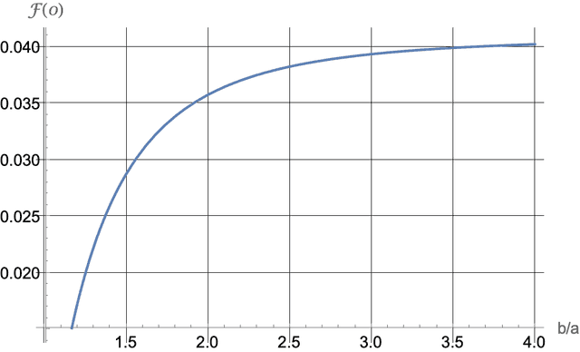
Figure 4. The force factor at z=0 as a function of the outer radius for $\lambda$=100. See equation (8) in the Appendix.

What is the bottom line?

To a very good approximation, $\mathcal{F}(z) \approx \mathcal{F}(0)$ for $-L/2 \leq z \leq L/2$. This validates the assertion that the magnetic force is proportional to the velocity inside the pipe.  Then we can write the magnitude of the force on the dipole as $$\begin{align}F(z) =\frac{ 9\sigma \mu _0^2 m^2 v }{8\pi}\mathcal{F}(0).\end{align}$$ The analytic expression for $\mathcal{F}(0)$ appears in the Appendix as equation (8) and is plotted in Figure 4 for $\lambda=L/a=100.$

The kinematics

We write the magnetic force on the dipole as $F=-\kappa~v$ and start with the differential equation $$M\frac{dv}{dt}=-\kappa~v+Mg~~~~\left(\kappa \equiv \frac{ 9\sigma \mu _0^2 m^2}{8\pi}\mathcal{F}(0)\right)$$ where $M$ is the mass of the dipole.

We cast the well known solution in terms of the terminal velocity, $v_{\text{ter}}=\dfrac{Mg}{\kappa}$: $$v=v_{\text{ter}}+(v_0-v_{\text{ter}})e^{-g~t/v_{\text{ter}}}\implies e^{-g~t/v_{\text{ter}}}=\frac{(v-v_{\text{ter}})}{(v_0-v_{\text{ter}})}.$$

Also, $$z=\int_0^tv~dt=v_{\text{ter}}t+\frac{v_{\text{ter}}(v_0-v_{\text{ter}})}{g}\left[1-e^{-g~t/v_{\text{ter}}}\right].$$ By eliminating the exponential, the two equations can be combined to yield $$\begin{align}z=v_{\text{ter}}t-\frac{v_{\text{ter}}\left(v-v_0\right)}{g}.\end{align}$$

A suggested experiment

An obvious experiment to perform and analyze would be to drop a magnet into a pipe and use photogates and data logging software to measure the entry velocity $v_0$, exit velocity $v_{\!f}$, and transit time $T$. Equation (6) becomes $$\begin{align}L=v_{\text{ter}}T-\frac{v_{\text{ter}}\left(v_{\!f}-v_0\right)}{g}.\end{align}$$It can be solved to find the terminal velocity. Repeating for other choices of entry velocity should verify the constancy of the terminal velocity. The value of the terminal velocity would then determine the value of $\kappa.$  Note that this determination is based on kinematics and is independent of the magnet model.

Moreover, equation (5) shows that  the force factor (determined by the pipe geometry), and the conductivity (determined by the choice of pipe material), can be mathematically separated out of $\kappa.$  One can test the validity of this separation by performing a series of experiments in which the same magnet is dropped through pipes of various wall thicknesses, lengths, and conductivities. When $\mathcal{F}(0)$ and the conductivity are factored out of $\kappa$, a constant shared by all experimental runs should be left.  One can then solve equation (5) to find an effective magnetic moment appropriate to a given magnet.

As an aside and because there is no other suitable place in the article, the author cannot resist mentioning the following observation. With the standard definitions of average velocity $\bar v=L/T$, average acceleration $\bar a=(v_{\!f}-v_0)/T$ and exponential time constant $\tau=v_{\text{ter}}/g$, equation (7) becomes the curiously suggestive relation $$v_{\text{ter}}=\bar v+\bar a\tau.$$It brings together two explicit constants, $v_{\text{ter}}$ and $\kappa$, an implicit independent variable, $v_0$ and two implicit dependent variables, $v_{\!f}$ and $T$. Thus, despite its SUVAToid appearance, it is a constraint relation on the dependent variables.

Summary and afterthoughts

The magnetic dipole model of a magnet falling through a pipe is sufficient to show mathematically that the magnetic force opposing the motion of the falling dipole inside the solenoid is fast-rising and can be written as a constant $\kappa$ multiplied by the instantaneous velocity.  The model also affords the calculation of a force factor that allows the separation of the pipe geometry and conductivity from the constant $\kappa.$ Once that separation is done, one may extract a value for an effective dipole moment that could serve as input to a more realistic model than the point dipole.

Furthermore, if a realistic model is a goal, it seems that a good place to focus one’s experimental efforts are the entry and exit points of the magnet. As Figure 3 shows, at these points, the force profile is most sensitive to the shape of the magnet and its effective range. Whatever one’s goal, the point dipole model has quite a bit to say; its simplicity makes it a good place to start the mathematical analysis of a magnet falling through a conducting pipe.

Acknowledgment

The author wishes to thank user @Delta2 for helpful comments and remarks on an earlier version of this article.

Appendix

With reduced lengths $\lambda= L/a$ and $\beta = b/a$, the value of the force factor is

$$\begin{align}\mathcal{F}(0)= & \frac{\lambda}{96a^3}\left[\frac{80 \beta ^4-32 \beta ^2 \lambda ^2-5 \lambda ^4}{\beta ^2 \left(4 \beta ^2+\lambda ^2\right)^3}-\frac{80-32 \lambda ^2-5 \lambda ^4}{\left(\lambda ^2+4\right)^3}\right] \nonumber \\ & + \frac{5}{192a^3}\left[\tan ^{-1}\left(\frac{\lambda }{2}\right)-\frac{1}{\beta ^3}\tan ^{-1}\left(\frac{\lambda }{2 \beta }\right)\right]
.\end{align}$$

References

For readers who wish to explore other approaches. The list is not meant to be complete.
C.S. MacLatchy, P. Backman and L. Bogan,  Am. J. Phys.  61, 1096 (1993); doi: 10.1119/1.17356
K.D. Hahn, E.M. Johnson, A. Brokken and Steven Baldwinc,  Am. J. Phys.  66,  1066 (1998); doi: 10.1119/1.19060
Y. Levin, F.L. da Silveira and F.B. Rizzato,  Am. J. Phys. 74, 815 (2006); doi: 10.1119/1.2203645
G. Donoso, C.L. Ladera and P. Martin,  Eur. J. Phys.  30 (2009),  855–869 doi:10.1088/0143-0807/30/4/018