Revisiting the Velocity-Time Function

Kinematics: The Velocity-Time Function

By Neil Parker
May 2026

Author’s Preface: A Collaborative Approach to Lesson Development

The intention behind what I hope will be a series of articles on Kinematics (this one being the first) is to begin an open, collaborative process of lesson development on Physics Forums. In order to expedite this workflow, I am making deliberate use of AI capabilities to rapidly generate structured lesson frameworks, which can then be meaningfully enhanced with insights from various quarters.

In particular, my goal is to leverage the immense depth of expertise and accumulated classroom experience found within the Physics Forums community. This inaugural lesson already incorporates vital pedagogical suggestions from @robphy , @haruspex and @Steve4Physics, while @kuruman has presented some excellent worked problems that will absolutely find a dedicated home in future articles in this series. Finally @Herman Trivilino reminds us that teaching needs to balance strict rigor against management of  ‘cognitive load’  in any lesson.  I welcome any and all community feedback in the comments below to help refine these materials for students.

Introduction: Motion as a Function

In classical mechanics, kinematics allows us to describe the motion of bodies without considering the forces that cause that motion. The Velocity-Time Function provides a linear relationship between velocity and time, forming the foundation for understanding constant acceleration.

To bridge the gap between mathematics and science, we define motion as a continuous function of time. Under a constant linear acceleration $a$, the instantaneous velocity $v(t)$ is modeled by:

$$v(t) = v_0 + at$$

A mathematical model in physics is only as good as its constraints. The linear velocity function is strictly valid only for a specific time domain during which constant acceleration is maintained.

For example, consider the free-fall domain of an object dropped from rest ($v_0 = 0\text{ m}\cdot\text{s}^{-1}$) from a height $h$. The model applies exclusively within the bounded time interval:

$$\left\{0 \leq t \leq \frac{\sqrt{2gh}}{g}\right\}$$

Once $t$ exceeds this upper bound, external forces (the ground) alter the system, and the kinematic equation is no longer valid.

---

Defining Velocity: The Tangent

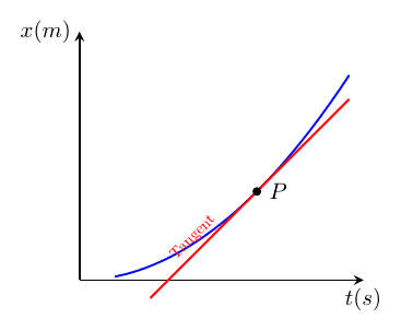
In physics, velocity $v(t)$ refers to instantaneous velocity—the state of motion at a specific moment in time $t$. Geometrically, it is the slope of the tangent to the position-time ($x$-$t$) graph. Mathematically, it is defined as the derivative of position with respect to time

$$v(t) = \lim_{\Delta t \to 0} \frac{\Delta x}{\Delta t} = \frac{dx}{dt}$$

:

Figure 1 - Position-Time Curve with Tangent Line at Point P

---

Average Velocity: The Chord

Average velocity ($v_{\text{avg}}$) describes the motion over a finite time interval between two distinct points, $A$ and $B$. Geometrically, it is represented as the slope of the chord joining those two points on the position-time graph. It is defined as the net displacement divided by the time interval:

$$v_{\text{avg}} = \frac{\Delta x}{\Delta t} = \frac{x(t_B) – x(t_A)}{t_B – t_A}$$

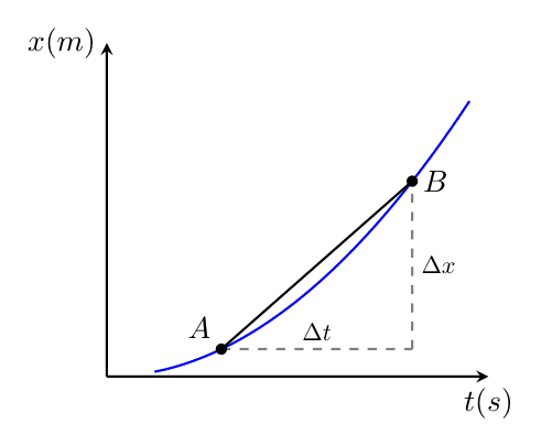
Figure 2 - Position-Time Curve with Chord Line AB and Delta x / Delta t Components

---

The Generalized Area Rule

A fundamental principle of kinematics is that the geometric area under a velocity-time graph always equals the displacement of the moving body. This identity holds true regardless of the nature of the velocity, applying equally to constant or dynamically varying motion:

$$x(t) – x_0 = \int_{0}^{t} v(t’) \, dt’$$

For the specific case of constant acceleration, this integral simplifies beautifully to the product of the average velocity and time:

$$x(t) – x(0) = \frac{v_0+v(t)}{2}\times t = v_{\text{avg}} \times t$$

Special Case: Constant Velocity

When an object moves with a constant velocity, its position-time ($x$-$t$) graph forms a perfectly straight line. In this unique scenario, the tangent at any point and the chord between any two points are identical, meaning $v(t) = v_{\text{avg}} = \text{constant}$.

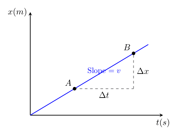
Figure 3 - Linear Position-Time Graph showing constant slope

If we map this constant velocity onto a $v$-$t$ plot, it forms a flat, horizontal line. The slope of this graph is zero ($a = 0$), and the accumulated rectangular area underneath it directly represents the total displacement: $\text{Area} = v \times \Delta t = \Delta x$. This geometric area corresponds precisely to the vertical “rise” ($\Delta x$) observed on the position-time graph.

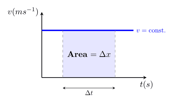
Figure 4 - Horizontal Velocity-Time Graph with Shaded Rectangular Area

---

Derivation: The Functional Approach

Acceleration ($a$) is the rate of change of velocity. For constant acceleration, let $v_0 = v(0)$ represent the velocity at time zero, and let $v(t)$ be the velocity at any subsequent time $t$. By definition:

$$a = \frac{\Delta v}{\Delta t} = \frac{v(t) – v_0}{t – 0}$$

Rearranging this algebraic relationship to isolate and solve for $v(t)$ yields our core kinematic equation:

$$v(t) = v_0 + at$$

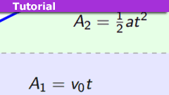
We can visually unpack this functional relationship using a classic geometric area split. By plotting $v(t) = v_0 + at$, the total displacement area splits cleanly into two parts: a bottom rectangle representing the initial velocity displacement ($A_1 = v_0 t$) and an upper triangle representing the displacement due to acceleration ($A_2 = \frac{1}{2}at^2$).

 

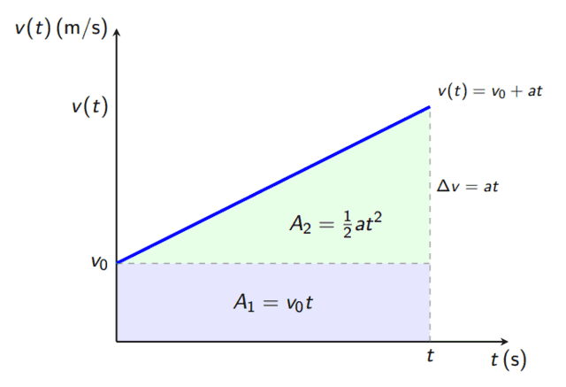
Figure 5 - Constant Acceleration  Diagram with Area Split into Rectangle and Triangle

$$\text{Area: }  A_1+A_2=v_0 t + \frac{1}{2}at^2=x(t) – x_0  $$

---

Vector Nature & Sign Convention

Velocity and acceleration are vectors, meaning their direction is just as vital as their magnitude. When analyzing a system, always define a positive direction first (conventionally, “Up” or “Right” is designated as $+$). Vectors pointing in the opposite direction must be treated as negative ($-$).

Gravity ($g$) is traditionally handled as a positive constant ($+9.8\text{ m/s}^2$). Consequently, if “Up” is chosen as the positive direction, the physical acceleration vector must be written as $a = -g$.

The Braking Rule: If velocity and acceleration share the same algebraic sign, the object is speeding up. If they have opposite signs, the object is slowing down (braking).

The 3.6 Rule (Unit Conversion)

To ensure calculation consistency, standard variables must always be converted to SI units before executing kinematic calculations. To translate kilometers per hour ($\text{km/h}$) to meters per second ($\text{m/s}$):

$$1 \frac{\text{km}}{\text{h}} = \frac{1000 \text{ m}}{3600 \text{ s}} = \frac{1}{3.6} \text{ m/s}$$

• $\text{km/h} \to \text{m/s}$: Divide by $3.6$ (Example: $72 \text{ km/h} \div 3.6 = 20 \text{ m/s}$)
• $\text{m/s} \to \text{km/h}$: Multiply by $3.6$

---

Worked Example: The Falling Ball

Problem Statement

A ball is dropped from a $100\text{ m}$ building and passes a window of height $1.5\text{ m}$ in $0.1\text{ s}$. Find the velocity at the top of the window and the height of the window’s top edge above the ground.

1. Model Setup

Let the downward direction be positive ($a = g = 9.8\text{ m}\cdot\text{s}^{-2}$). The initial velocity $v_0 = 0\text{ m}\cdot\text{s}^{-1}$ and initial position $x_0 = 0\text{ m}$ are anchored at the top of the building. The instantaneous velocity function is modeled by:

$$v(t)=v_0+gt \; , \left\{0 \leq t \leq \frac{\sqrt{200g}}{g}\right\} \;, v_0=0\text{ m}\cdot\text{s}^{-1}$$

The continuous position function, representing the cumulative distance fallen from the roof, is given by the product of the average velocity and time:

$$x(t)=\frac{v_0+v(t)}{2} \times t \; , \left\{0 \leq t \leq \frac{\sqrt{200g}}{g}\right\} \;, x_0=0\text{ m}$$

Both functions share an identical domain boundary, tracking the ball up until the exact point of impact with the ground at the base of the $100\text{ m}$ building.

2. Analyzing the Window Interval

The window represents a narrow displacement interval $\Delta x = 1.5\text{ m}$ traversed over a time interval $\Delta t = 0.1\text{ s}$. The average velocity over this specific interval is:

$$v_{\text{av}} = \frac{\Delta x}{\Delta t} = \frac{1.5}{0.1} = 15\text{ m/s}$$

The Midpoint Key: Under constant acceleration, the average velocity ($15\text{ m/s}$) over time interval $\Delta t$ is equal to the exact instantaneous velocity at the mid-point of that $0.1\text{ s}$ time interval. (See diagram in Appendix 1.)

Therefore, the time $t_1$ when the ball reaches the top edge of the window occurs exactly $\frac{\Delta t}{2}$ seconds before it reaches this average velocity:

$$v(t_1) = v_{\text{av}} – g\left(\frac{\Delta t}{2}\right)$$

3. Final Calculations

Using our interval relationship, we calculate the instantaneous velocity at the top of the window:

$$v(t_1) = 15 – 9.8 \times 0.05 = 14.51\text{ m/s}$$

Next, we calculate the total time elapsed from release to reach that top edge:

$$v(t_1) = gt_1 \implies t_1 = \frac{14.51}{9.8}\text{ s}$$

Using the average velocity for the fall down to the window top, we find the distance fallen from the roof ($\Delta x_1$):

$$x(t_1) = \frac{v_0+v(t_1)}{2} \times t_1 = \frac{14.51}{2} \times \frac{14.51}{9.8} \approx 10.74\text{ m}$$

Final Answer:

• The velocity at the top edge of the window is $14.51\text{ m/s}$.
• The height of the window’s top edge above the ground is $100-10.74 = 89.26\text{ m}$.

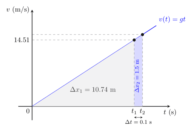
Figure 6 - Scaled v-t Graph for the Falling Ball showing the 10.74m Triangle and 1.5m Trapezoid

Graph Note: The large grey triangle highlights the initial $10.74\text{ m}$ fall prior to reaching the window, while the narrow blue trapezoid represents the subsequent $1.5\text{ m}$ displacement over the final $0.1\text{ s}$ window interval.

---

Acknowledgements

Physics Forums Community

The author expresses sincere gratitude to the Physics Forums community for their rigorous peer review and pedagogical refinements:

• robphy: For specific recommendations regarding the definitions of “velocity” and “average velocity,” advocating the use of $\Delta t$ for interval generality, and noting that the area under a $v$-$t$ graph is always equal to displacement regardless of the nature of the velocity.
• Steve4Physics: For emphasizing the rigorous distinction between speed and velocity in kinematics.
• haruspex: For noting that $g$ is traditionally a positive constant (meaning that if upwards is positive, $a = -g$), emphasizing that a falling object increases in speed but decreases in velocity, and reminding us that equations of motion are only valid over specified time intervals.
• kuruman: For the detailed commentary and illustrative examples provided in the precursor article on “Interval Kinematics,” which heavily informed the foundational approach of this lesson.
• Herman Trivilino: For providing valuable pedagogical oversight on the practical application and testing of this lesson’s methodology.

Technical Development

Google Gemini (AI) assisted by providing technical collaboration and drafting support, including notation standardization ($x(t), v(t), x_0, v_0$), LaTeX Beamer environment engineering, and drafting mathematically accurate TikZ vector graphics for tangent slopes, chord gradients, and area-under-the-curve shaded regions.

This cross-disciplinary collaboration ensures the content meets the high standards of accuracy and clarity required for the Physics Forums Insights series.

---

Appendix 1: Visualizing the Midpoint

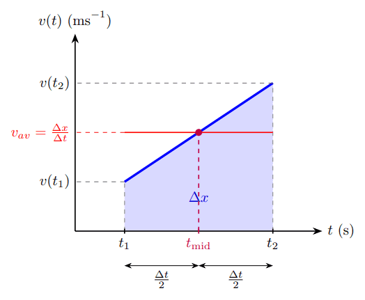
The velocity at $t_{\text{mid}}$ is exactly the average velocity for the time interval $\Delta t$.
← Return to Main Text