Video Analysis of Spheres Falling Through Two Liquids

Introduction

Providing accurate fluid-dynamics experiments for undergraduate laboratories is challenging in several ways, including reproducibility, simplicity, and accessibility for introductory students. Data from many introductory experiments, for example, are not sufficiently precise to decide whether a linear or quadratic relationship better models the dependence of drag force on velocity.

An optimal laboratory experiment is inexpensive enough for multiple student groups to perform and produces accurate, repeatable results. Examples are plentiful in undergraduate kinematics labs (simple harmonic oscillators, sliding-block experiments), but cost-effective and accurate experiments in fluid dynamics are less common.

High-frame-rate video cameras (60–240 fps) are now widely available, enabling cost-effective, accurate fluid-dynamics experiments. This article provides one such example and explains the precautions needed to obtain accurate dynamics using common, inexpensive materials. Simple lead and steel spheres are dropped through stacked layers of canola oil and glycerine in a clear graduated cylinder. The two-layer design provides ample data for developing and testing predictive models: spheres accelerate in the canola oil and decelerate after transitioning into the more viscous glycerine.

Table 1: Diameter and mass for four spheres used in the experiment. All digits may not be significant but are included to reduce rounding errors in anticipated predictive modeling.

Method

Apparatus

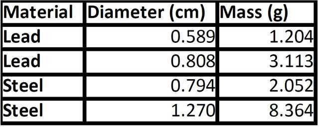
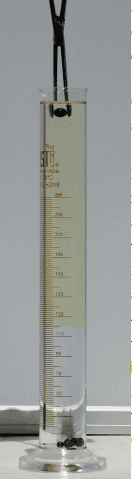
Four different spheres of known diameter and mass (Table 1) were individually suspended with forceps near the top of a graduated cylinder containing canola oil over glycerine, then released to pass through both fluids before reaching the bottom. Liquid depths were chosen as a compromise between the height of the available graduated cylinder and giving the smaller spheres enough distance to approach near-terminal velocity in each liquid. The graduated cylinder and liquids are shown in Figure 1.

Pilot testing showed that releasing a sphere from air often causes an air bubble to attach and travel with the sphere for 5–10 cm into the liquid, significantly altering the net force and the resulting dynamics. Releasing the sphere from a position slightly immersed in the top liquid eliminates this confounding factor and produces more consistent data.

Video recording and analysis

A Nikon CoolPix B500 recorded each trial at 120 frames per second. Videos were downloaded to a computer and imported into the free video-analysis program Tracker (version 5.1.1). Raw position‑vs‑time data were exported to a spreadsheet. Velocity‑vs‑time was then computed in the spreadsheet as described below.

Figure 1: Graduated cylinder including forceps, sphere, canola oil (golden upper liquid), and glycerine (lower liquid). The glycerine layer is approximately 10 cm thick, and the canola layer is approximately 20 cm thick.

Video best practices (laboratory procedures)

Over years of use, our lab has developed practical procedures to improve accuracy in video kinematics. The main procedures applied in this experiment were:

1. Mount the camera on a tripod (camera fixed, not handheld).
2. Keep motion in a single plane as nearly equidistant from the camera as possible. Placing the camera farther away reduces perspective curvature; here the camera was ~3 m from the ~30 cm vertical motion.
3. Use zoom so the motion fills the frame and uses as many pixels as possible for tracking.
4. Orient the camera so more pixels lie along the dominant motion direction (portrait for vertical motion used here).
5. Use the brightest practical lighting to enable fast shutter speeds (these videos were taken outdoors in direct sunlight).
6. Place the camera near the center of the motion to minimize parallax. For vertical motion here, cylinder graduations were used to position the camera at the vertical center.
7. Calibrate using a known length scale as close as possible to the plane of motion. Length scales significantly closer or farther from the motion introduce calibration errors; here, the cylinder graduations served as the scale.
8. Manual tracking is often more accurate than automated trackers when resolution is limited or optical distortion exists. Stepping through frames and recording the object’s position manually typically takes 5–10 minutes per video but can yield more accurate positions.
9. Decide whether to track the object’s leading edge or its center. For symmetric objects in limited-resolution, distorted images (appearing elliptical), the center is usually more reliable. For blurred images (slower shutter speeds), the leading edge can be more consistent.
10. Avoid opaque black-box velocity/acceleration routines. Export raw position‑vs‑time data to a spreadsheet for transparent analysis.
11. Compute a “local” slope for velocity using multiple nearest neighbors (3–7 points) rather than simple nearest‑neighbor differences. Here, five points were used with the spreadsheet SLOPE() function as an acceptable trade-off between instantaneous velocity and smooth, physically reasonable variations.
12. Velocity data provide stronger tests of experimental/analysis techniques and predictive models than position data, because many models can visually match position but diverge in velocity.
13. Balance frame rate and spatial resolution. Pilot testing here showed each trial lasted <0.5 s in a liquid layer. Using 120 fps gave sufficient temporal resolution (~20–60 points per liquid) at 640‑pixel width; sacrificing frame rate to increase spatial resolution did not improve accuracy for this design.
14. When using Tracker manually, calibrating in centimeters rather than meters often yields more precise cursor readouts.
15. Determining t = 0 can be difficult. If the first frames show velocity increasing approximately linearly, perform a least‑squares fit of velocity vs. time for the earliest frames and shift the time axis so the fitted line extrapolates to v = 0 at t = 0. This compensates for any small release impulse.

Density measurement for buoyancy

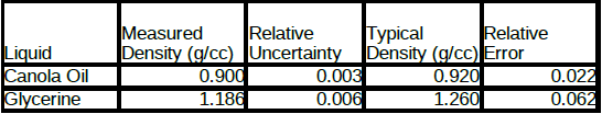
Predictive models require accurate fluid densities to compute buoyant forces. At the experiment temperature (28 °C), the densities of canola oil and glycerine were measured by recording the mass of each fluid at 10 equal-volume increments in a graduated cylinder on a calibrated digital scale and performing a linear least‑squares fit; density is the slope of mass vs. volume.

With distilled water this technique agrees with accepted values to within 0.1% — this represents the uncertainty in the slope measurement with distilled water. Uncertainties for canola oil and glycerine are larger (likely due to their higher viscosities), and measured densities can differ noticeably from typical reference values because consumer products vary in composition and purity. For modeling, use the densities measured in the experiment rather than standard textbook values.

Table 2: Densities of canola oil and glycerine needed for predictive modeling. The relative uncertainty is computed from the reported uncertainty in the best-fit slope. The relative error is computed from the difference between typical reported densities and the measured density reported here.

Figure 2: Velocity vs. time for 1.204 g lead sphere.

Results

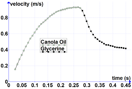
Figure 2 shows velocity vs. time for the smaller lead sphere. The sphere accelerates from rest while approaching a near-terminal velocity of ≈0.93 m/s in canola oil. As expected, the sphere slows upon entering the more viscous glycerine and approaches a near-terminal velocity of ≈0.4 m/s there.

Velocity vs. time data for all four spheres are provided in Table 3 to support predictive modeling. Position vs. time data are omitted to encourage modeling comparisons using velocity (a more discriminating metric) rather than position, since many models can visually match position while differing in velocity.

Analysis and modeling

1.204 g Lead		3.113 g Lead		2.052 g Steel		8.364 g Steel
time (s)	v (m/s)	time (s)	v (m/s)	time (s)	v (m/s)	time (s)	v (m/s)
0.0245	0.1548	0.0292	0.1992	0.0438	0.2424	0.0313	0.2040

Table 3: Velocity vs. time data for four spheres. The data point corresponding to the first frame showing the sphere in the glycerine is shown in bold. All digits shown may not be significant, but are shown to allow comparisons with modeling, including more accurate computations of RMS errors for different predictive models.

Discussion

Many smartphones already provide frame rates comparable to the dedicated camera used here (120 fps). The accuracy of the experiment depends more on careful technique than on expensive equipment. The two-layer liquid configuration permits quantitative observation of both positive and negative accelerations within a single trial. Observations show the transition between liquids is relatively clean: canola oil is not significantly dragged into the glycerine. This contrasts with dropping spheres from air, where an attached air bubble can distort the motion.

Tracking data from lead spheres was generally more uniform than for shiny steel spheres. Shiny steel reflects light and complicates optical tracking; painting or otherwise making steel spheres a dark, matte color (before measuring diameter and mass) is recommended to improve tracking accuracy.

Typical uncertainties in the velocity determination for most data points are between ~0.5% and 2.0%, estimated from uncertainties in the slope of position vs. time. Higher frame rates or resolution will not necessarily improve accuracy if the primary limitation is the camera sensor’s pixel-to-distance linearity. To evaluate a camera’s accuracy potential, drop a lead sphere in air over 0.5–0.75 m and use a least‑squares quadratic fit of height vs. time to estimate g; comparison with the known g gives a practical sense of the camera’s achievable accuracy. Most consumer cameras of reasonable quality yield accuracy potential in the 0.5%–2% range when due care is taken.

Students gain the most educational value by repeating a similar experiment and practicing the due-care procedures described here. Alternatively, sufficient data are provided for theoretical modeling: fit a model to one trial (for example, treat fluid viscosities as adjustable parameters) and test it against the other trials by computing RMS differences without additional tuning. Models that assume linear or quadratic drag dependence can be discriminated quantitatively by comparing RMS errors between predicted and measured velocity curves.

Comment Thread