Dark Energy Part 3: Fitting the SCP Union 2.1 Supernova Data

In Part 1 of this 3-part series, I explained kinematics in Einstien-deSitter (EdS) cosmology and in Part 2, I explained kinematics in $\Lambda$CDM cosmology (essentially EdS plus a cosmological constant $\Lambda$). Now I will bring those models to bear on the Supernova Cosmology Project (SCP) Union2.1 type Ia supernova data. This will show clearly how the EdS fit of the supernova data is greatly improved by adding $\Lambda$ to Einstein’s equations (EEs) of general relativity (GR). This fact convinced the astronomy community that a cosmological constant is indeed needed in EEs. This cosmological constant $\Lambda$ is often referred to as “dark energy,” as I explained in Part 2. I’ll start by explaining the concept of “distance modulus.”

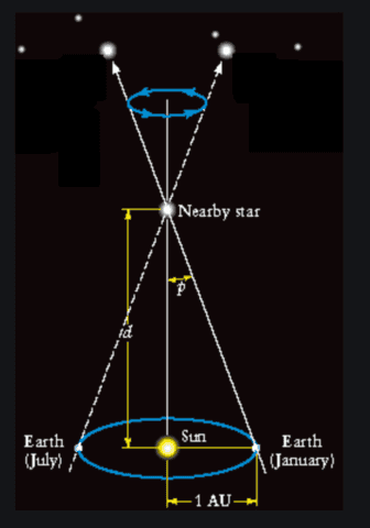
In order to obtain distances in astronomy, astronomers use the “cosmic distance ladder.” That is, they obtain farther distances using information obtained at smaller distances. For example, using the Earth-Sun distance astronomers measure the parallax angle to relatively nearby stars to obtain the distance to those stars (see picture below and this Insight by Janus). The distance to a star with a parallax angle of one arcsecond is defined to be 1 parsec (pc). Using the known Earth-Sun distance you can compute 1pc = 3.26cy (again, read “cy” as “light-years”). They can use this method on thousands of stars in our galactic neighborhood. Once they know how far away a star is, they can figure out how intrinsically bright it is, i.e., how bright it would appear at a particular reference distance (chosen here to be 10pc). Doing that for many stars allows them to build a table of information on types of stars (called the H-R diagram).

Now, when they see a star of a particular type that is too far away to exhibit a measurable parallax angle, they can deduce its distance by using its intrinsic brightness from the H-R diagram (given a number $M$ called its “absolute visual magnitude,” as I will explain below) and comparing that to its apparent brightness (given a number $m$ called its “apparent visual magnitude,” as I will explain below). This method is good as long as you know an object’s intrinsic brightness and the object is bright enough to be seen at all. It turns out that for your average star this method isn’t good for cosmological distances because stars just aren’t bright enough to be seen at cosmological distances. What Perlmutter, Schmitt, and Riess did to win the 2011 Nobel Prize in Physics was to figure out $M$ for a very bright object that can be seen billions of light-years away — the type Ia supernova. Specifically, they were able to obtain the “distance modulus” $m\, – M$ and redshift for hundreds of distant supernovae. That is the SCP Union2.1 data I will fit using EdS and $\Lambda$CDM kinematics obtained in Parts 1 and 2 of this series. To get started, I need to explain distance modulus quantitatively.

The apparent visual magnitudes $m_1$ and $m_2$ of two objects with luminosities $L_1$ and $L_2$, respectively, are related by this equation

\begin{equation} m_1 – m_2 = -2.5 \log{\left(\frac{L_1}{L_2}\right)} \label{m1m2} \end{equation}

This is defined so that when $m_2$ is larger than $m_1$ by 5, $L_1 = 100L_2$. You will notice that this seems backwards because the larger the apparent visual magnitude, the dimmer (less luminous) the object appears. That obtains for historical reasons. Apparently, long ago, astronomers ranked stars with the brightest stars being ranked the highest and that system became the magnitude system. Ugh. Anyway, this magnitude system is used to find the distance to an object by using Eq. (\ref{m1m2}) for one object at two distances. Since luminosity (power per unit area) goes as $\frac{1}{d^2}$ we have

\begin{equation} m_1 – m_2 = -2.5 \log{\left(\frac{d_{2}^2}{d_{1}^2}\right)} \label{d1d2} \end{equation}

Now if we’re talking about the apparent visual magnitude ($m$) of one object at an unknown distance $d$ compared to its apparent visual magnitude ($M$) at a known reference distance 10pc, then we have

\begin{equation} \mu := m\, – M = 5 \log{\left(\frac{d}{10pc}\right)} \label{mu1} \end{equation}

where $\mu$ is called the “distance modulus.” In cosmology, this luminosity distance $d$ is related to the proper distance $r_o$ by $d = (1+z)r_o$, so when using a particular cosmology model we have

\begin{equation} \mu = 5 \log{\left(\frac{(1+z)r_o}{10pc}\right)} \label{mu} \end{equation}

We obtain $r_o$ as a function of $z$ (redshift) and $t_o$ (age of the universe) in EdS cosmology while we obtain $r_o$ as a function of $z$, $t_o$, and $\Omega_m$ (or equivalently, $\Omega_\Lambda$) in $\Lambda$CDM cosmology. Therefore, the Union2.1 data ($\mu$ versus $z$) is to be fit using $t_o$ in EdS cosmology while it is fit using $t_o$ and $\Omega_m$ (or equivalently, $\Omega_\Lambda$) in $\Lambda$CDM cosmology. We found

\begin{equation} r_o = 3ct_o\left(1 – \frac{1}{\sqrt{1+z}}\right) \label{EdSro}\end{equation}

for EdS cosmology and

\begin{equation} r_o = \frac{ct_o}{H_ot_o}\int_{a_e}^{1}\frac{da}{a\sqrt{\frac{\Omega_m}{a} + \Omega_\Lambda a^2}}  \label{Lambdaro} \end{equation}

for $\Lambda$CDM cosmology. I will enter $t_o$ in Gy and $r_o$ in Gcy for both models. Eq. (\ref{mu}) is then

\begin{equation} \mu = 5 \log{\left(\frac{(1+z)r_o}{3.26}\right) + 40} \label{mu2} \end{equation}

The data can be obtained at the Supernova Cosmology Project website (see “Union2.1 Compilation Magnitude vs. Redshift Table (for your own cosmology fitter)” in “Cosmology Tables”). I have the relevant data in this txt file and this xlsx Excel file. In both cases, $z$ is column 1 and $\mu$ is column 2. Here is my MATLAB code for doing the comparison fits:

%First I import my data. Note that your Workspace in MATLAB will have to contain the proper file names.
z = table2array(SCPUnion2);
mu = table2array(SCPUnion1);

%We need to transpose the data into columns as it was imported as rows.
z = z’;
mu = mu’;

%These are the two functions in the scaling factor “a” that I will be integrating. Om is $\Omega_m$ and OL is $\Omega_\Lambda$.
Afunc = @(a,Om,OL) 1./sqrt(Om./a + OL*a.^2);
Rfunc = @(a,Om,OL) 1./sqrt(Om.*a + OL*a.^4);

%Here are the best fit $\Omega$ values for the $\Lambda$CDM fit shown.
%I varied $\Omega_m$ to 3 sig figs to find the smallest root mean square error (RMSE) for the $\Lambda$CDM fit (I found 6.3963).
Om = 0.283;
OL = 1 – Om;

%Here are the ages of the universe for $\Lambda$CDM and EdS, respectively, used for the fits.
%I varied the EdS value to 3 sig figs to find the smallest RMSE for the EdS fit (I found 8.1897).
%I did not vary $t_o$ for $\Lambda$CDM. Since EdS has only one fitting parameter I wanted
%$\Lambda$CDM to have only one fitting parameter ($\Omega_m$). In reality, both would be varied of course.
to = 13.82;
toEdS = 10.8;

%This is the numerical integral for $H_o$ times $t_o$.
Hoto = integral(@(a) Afunc(a,Om,OL),0,1);

%This is $a_e$ for each of the 580 values of $z$.
ae = 1./(1 + z);

%This loop computes $r_o$ for the $\Lambda$CDM model for all 580 values of $z$.
for ii = 1:580
Ro(ii) = to*integral(@(a) Rfunc(a,Om,OL),ae(ii),1)/Hoto;
end

%This computes $r_o$ for the EdS model for all 580 values of $z$.
RoEdS = 3*toEdS*(1 – 1./sqrt(1 + z));

%Here are the theory values for $\mu$.
TheoryMuLCDM = 5*log10((1 + z).*Ro/3.26) + 40;
TheoryMuEdS = 5*log10((1 + z).*RoEdS/3.26) + 40;

%I am using root mean square error for obtaining the best fit.
RMSE_LCDM = sqrt(sum((TheoryMuLCDM – mu).^2))
RMSE_EdS = sqrt(sum((TheoryMuEdS – mu).^2))

%This is where I do my plots (shown below).
plot(z,mu,’o’,’color’,’black’)
hold
plot(z,TheoryMuLCDM,’*’,’color’,’red’)
plot(z,TheoryMuEdS,’*’,’color’,’green’)
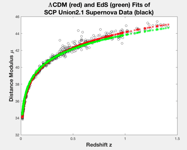
title({‘\LambdaCDM (red) and EdS (green) Fits of’;’SCP Union2.1 Supernova Data (black)’},’FontSize’,17,’FontWeight’,’bold’)
xlabel(‘Redshift z’,’FontSize’,15,’FontWeight’,’bold’)
ylabel(‘Distance Modulus \mu’,’FontSize’,15,’FontWeight’,’bold’)
hold off

Using RMSE is a crude way to determine the best fit, but it results qualitatively in precisely what is publicized about the role of $\Lambda$. That is, $\Lambda$ plus EdS produces a greater $\mu$ at large redshifts than EdS alone (see my plots below). This discovery by Perlmutter, Schmitt, and Riess caused quite a stir in astronomy when it was announced in 1998, but today the use of $\Lambda$ in the concordance model for cosmology is unquestioned. The quantum source of this so-called “dark energy” remains a mystery however.

Comment Thread