
How to Get Started with Bayesian Statistics
Table of Contents
Confessions of a moderate Bayesian, part 1
Bayesian statistics by and for non-statisticians
https://www.cafepress.com/physicsforums.13265286
Background
I am a statistics enthusiast, although I am not a statistician. My training is in biomedical engineering, and I have been heavily involved in the research and development of novel medical imaging technologies for the bulk of my career. Due to my enjoyment of statistics and my professional research needs I was usually the author in charge of the statistical analysis of most of our papers.
In the course of that work, I developed an interest in and an appreciation of Bayesian statistics, which I have used in the analysis of most of my more recent projects. I have published the Bayesian analysis of some of these studies, although more were done in addition to standard (published) frequentist analysis.
This article will be a quick and practical how-to on getting started doing Bayesian statistics. I will leave the whys and wherefores to a future Insight. Except, I will say that my main motivation is that I find that the results of the Bayesian methods are more in line with how I think about science.
Software
The best software for general-purpose statistics is R: It is free. It has a large ecosystem of packages. It is free. Most new statistical methods are implemented in R first. It is free. It has more well-tested features than any other statistical system. It is free. It has a huge user community with lots of advice, tutorials, and guides. And finally, it is free.
Scientific programming in R usually goes like this:
- Find a package in R that already does what you want
- Run the package on your data
- Publish the results
If you are planning on using R in your scientific work, please be sure to use its citation() function to properly credit both the developers of R and any packages that you use in your research. They have provided it free to us, so a bit of gratitude and scientific recognition is the least that we can do.
IDE
I use RStudio which is probably the dominant IDE for R. It has basic console and code file capabilities, as well as graphing, help, and data navigation features.
The most important feature of RStudio is its built-in package management. With just a couple of clicks, you can download any available R package. It comes with the most common ones pre-installed. Start with RStudio and then download the packages through the IDE.
Graphics
One of the most important statistical tools is your own eyes and plotting data in a variety of different ways. I use the ggplot2 package for graphing, and many other graphing packages are based on it. I also use GGally and Bayesplot for additional convenient plotting features.
Bayesian statistics
Bayesian statistics is still rather new, with a different underlying mechanism. Most of the popular Bayesian statistical packages expose underlying mechanisms rather explicitly and directly to the user and require knowledge of a special-purpose programming language. This is good for developers, but not for general users. In contrast, commonly used frequentist packages usually hide this implementation-level detail from the general user.
To achieve widespread adoption of Bayesian techniques, what is needed is a “Bayesian version” of common statistical tests, with the implementation level hidden as much as possible. The best package I have found with that design philosophy is rstanarm. This package implements the most common statistical models with nearly identical interfaces as the frequentist version. It also has a rich Bayesian feature set including many posterior predictive features.
How to
To start, let’s load some libraries and data that we will use in this brief demo. The data we will use is the built-in “ChickWeight” data set. This records the weight of 50 chickens on one of 4 different diets from 0 days to 21 days old. The first diet is the control diet and then diets 2-4 are various experimental diets.
library(rstanarm)

library(ggplot2)

library(bayesplot)

library(emmeans)

data("ChickWeight")
Let’s take a brief look at the data by plotting it with ggplot
ggplot(data = ChickWeight, aes(x=Time,y=weight,color=Diet)) +

geom_jitter(size=3, alpha=0.4) +

geom_smooth(method="lm",se = FALSE) +

labs(title="Chick weights from 0 to 21 days", y = "Weight (g)", x = "Time (days)")
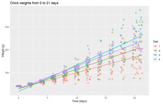
It looks like the variance of the data depends strongly on time. Perhaps more importantly, the linear fits appear to have some bias for the first week. So we will remove the first week and transform the data to a log scale.
dat <- subset(ChickWeight,Time > 7)

ggplot(data = dat, aes(x=Time,y=weight,color=Diet)) +

scale_y_log10() +

geom_jitter(size=3, alpha=0.4) +

geom_smooth(method="lm", se = FALSE) +

labs(title="Chick weights from 7 to 21 days", y = "Weight (g)", x = "Time (days)")
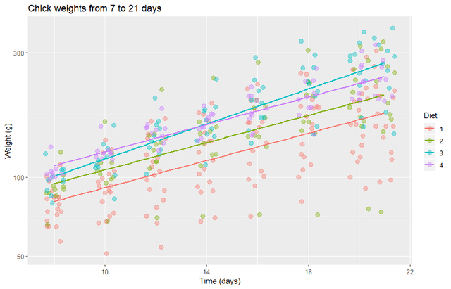
This produces a plot with a more nearly uniform variance and with no visibly obvious bias. It looks like most diets will have the same growth rate as the control diet, but diet 3 may have a higher growth rate. We will investigate this with both frequentist and Bayesian methods.
Frequentist analysis
We will run the data through a basic linear model fitting the log of the weights to the combination of the diet and the time.
fit <- lm( log(weight) ~ Diet * Time, data = dat)

summary(emmeans(fit, specs = trt.vs.ctrl ~ Diet|Time, type = "response"), infer = c(TRUE,FALSE))

summary(emtrends(fit, specs = trt.vs.ctrl ~ Diet, var = "Time"), infer = c(TRUE,FALSE))
This gives the following output
$`emmeans`

Time = 14.8:

Diet response   SE  df lower.CL upper.CL

1         121 2.63 372      116      127

2         142 4.11 372      134      150

3         170 4.90 372      160      180

4         167 4.88 372      157      177

contrast ratio     SE  df lower.CL upper.CL

2 / 1     1.17 0.0423 372     1.07     1.28

3 / 1     1.40 0.0506 372     1.28     1.52

4 / 1     1.37 0.0501 372     1.26     1.50
$`emtrends`

Diet Time.trend      SE  df lower.CL upper.CL

1        0.0599 0.00493 372   0.0502   0.0696

2        0.0601 0.00657 372   0.0472   0.0730

3        0.0768 0.00657 372   0.0639   0.0897

4        0.0602 0.00671 372   0.0470   0.0734

contrast estimate      SE  df lower.CL upper.CL

2 - 1    0.000149 0.00822 372 -0.01932   0.0196

3 - 1    0.016911 0.00822 372 -0.00255   0.0364

4 - 1    0.000304 0.00833 372 -0.01943   0.0200
Bayesian analysis
Duplicating the frequentist analysis
Now, we can do a Bayesian version of the same model. The calls are almost identical, with only one more argument for specifying the prior.
post <- stan_lm( log(weight) ~ Diet * Time, data = dat, prior = R2(.7))

summary(emmeans(post, specs = trt.vs.ctrl ~ Diet|Time, type = "response"), infer = c(TRUE,FALSE))

summary(emtrends(post, specs = trt.vs.ctrl ~ Diet, var = "Time"), infer = c(TRUE,FALSE))
The results of the Bayesian model are nearly identical to the frequentist results presented above.
$`emmeans`

Time = 14.8:

Diet response lower.HPD upper.HPD

1         122       117       127

2         142       134       151

3         169       160       179

4         166       156       176

contrast ratio lower.HPD upper.HPD

2 / 1     1.17      1.09      1.26

3 / 1     1.39      1.30      1.49

4 / 1     1.37      1.27      1.47
$`emtrends`

Diet Time.trend lower.HPD upper.HPD

1        0.0592    0.0502    0.0698

2        0.0595    0.0453    0.0719

3        0.0760    0.0629    0.0890

4        0.0595    0.0470    0.0728

contrast estimate lower.HPD upper.HPD

2 - 1    2.93e-04  -0.01536    0.0167

3 - 1    1.66e-02   0.00115    0.0322

4 - 1    6.88e-05  -0.01587    0.0159
Going beyond Bayes
So while it is great that we can essentially replicate the frequentist results, that in itself is not a particularly compelling reason to use Bayesian methods. So let’s now focus on some things that can be done with Bayesian statistics that either cannot be done at all with frequentist approaches or are rather unnatural/difficult.
Posterior parameter distributions
The first thing that is new and completely natural with Bayesian statistics is to look at the probability distribution of the model parameters. In this case, we will look at the differences in the slope of the regression lines, that is, the effect of the diets in increasing the rate of weight gain above the control diet.
mcmc_areas(post,pars = c("Diet2:Time","Diet3:Time","Diet4:Time"), prob = 0.8, prob_outer = 0.95) +

labs(title = "Posterior trends for weight gain", y="Probability density", x="log(weight gain (%/day))")
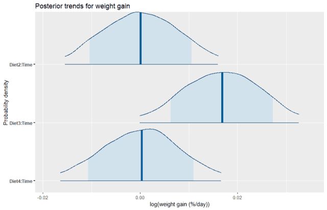
We can see that Diet2 and Diet4 have almost no average effect on the rate of weight gain, which is consistent with the plot of the data. Yet we also see that there is still some uncertainty, with about an 80% probability of being anywhere between positive and negative 1% weight gain per day relative to the control diet. In contrast, Diet3 looks like it is quite likely to have a higher rate of weight gain than the control. We can directly calculate the probability that the effect of Diet3 is less than zero by using the empirical CDF function as follows:
post.df <- as.data.frame(post)

ecdf(post.df$"Diet3:Time")(0)
This gives us only a probability of 0.019 that the effect is negative. Suppose instead that Diet3 is a more expensive diet, so it is only worth using if the improvement in the rate of weight gain is greater than about 1% per day (relative to the control). With a frequentist approach, this would require modifying the model and re-running the analysis, but here we can simply directly calculate it from the distribution as follows:
1-ecdf(post.df$"Diet3:Time")(0.01)
This gives us a probability of 0.802, so it seems like a good bet to go for the more expensive diet.
Posterior predictive simulations
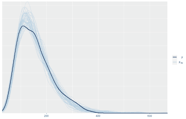
One of the things that I like best about Bayesian statistics is what is called posterior predictive sampling. You can use the model to generate simulated replicates of the data, which would be expected if you repeated the experiment. This simulation inherently accounts for the uncertainty in the model parameters. You can then compare the simulated replicates with the original data, and if the original data looks similar to the simulated replicates then you can conclude that the model is a good model for the data. So first we will generate 500 replicates:
w <- dat$weight

wrep <- exp(posterior_predict(post,draws = 500))
Once we have those 500 replicates then we can plot the probability density for the original data on top of the probability density for the first 50 replicates (or any other number). When we do so we see that the replicated data matches the distribution of the original data quite well
ppc_dens_overlay(w, wrep[1:50,])
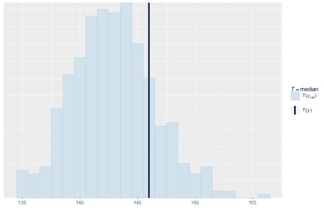
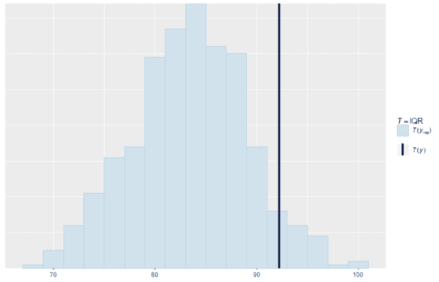
We can also look at standard summary statistics like the median and interquartile range and compare the summary statistic values replicates to the original data:
ppc_stat(w, wrep, stat = "median", binwidth = 1)

ppc_stat(w, wrep, stat = "IQR", binwidth = 2)
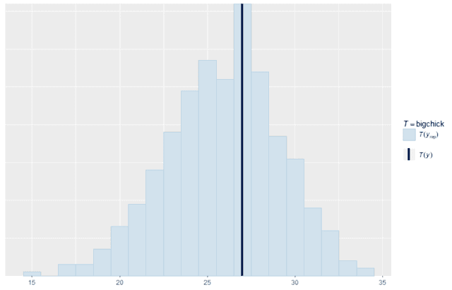
Custom statistics
We can also make custom summary statistics that are tailored for a specific application. For example, suppose that the most important thing to the business is increasing the number of chicks that weigh at least 200 g at 21 days old. We can write a summary function that counts exactly that quantity and compares the replicates with the original data. As you can see, the model replicates this specific quantity quite well. So for this purpose, it would be a good model to use. That may be more important than whether or not it accurately recreates the median.
bigchick <- function(x){

return(sum((dat$Time == 21)*(x>200)))

}

ppc_stat(w, wrep, stat = "bigchick", binwidth = 1)
Summary
So here we have seen a quick start to the basics of doing Bayesian statistics. This is based on my experience with a few different packages and performing these analyses on a few different research projects. Bayesian statistics has a philosophy and a meaning that I feel more closely represents the way that I think about science. But the main reason that I use Bayesian methods is because of how natural and easy it analyze the posterior parameters and the posterior predictive distributions.
I am not a statistician, so I am sure that my approach lacks a certain degree of statistical sophistication, but my experience with these tools has been enlightening for me and hopefully valuable for the PF community.
Continue to part 2: Frequentist Probability vs Bayesian Probability
Citations
- R Core Team (2018). R: A language and environment for statistical computing. R Foundation for Statistical Computing, Vienna, Austria. URL https://www.R-project.org/
- Goodrich B, Gabry J, Ali I & Brilleman S. (2020). rstanarm: Bayesian applied regression modeling via Stan. R package version 2.19.3 https://mc-stan.org/rstanarm
- Wickham. ggplot2: Elegant Graphics for Data Analysis. Springer-Verlag New York, 2016.
- Gabry J, Mahr T (2019). “bayesplot: Plotting for Bayesian Models.” R package version 1.7.1, <URL: https://mc-stan.org/bayesplot> .
- Russell Lenth (2019). emmeans: Estimated Marginal Means, aka Least-Squares Means. R package version 1.3.2. https://CRAN.R-project.org/package=emmeans
Education: PhD in biomedical engineering and MBA
Interests: family, church, farming, martial arts


”
This video might be interesting to people who read your Bayesian insights.
It would be great if you could take a look at it and share your thoughts:
[SIZE=4]”The medical test paradox: Can redesigning Bayes rule help?”[/SIZE]
[MEDIA=youtube]lG4VkPoG3ko[/MEDIA]
“Yes, [USER=5126]@Swamp Thing[/USER], I actually prefer that format of Bayes’ theorem also. I didn’t go into a lot of detail like this video, but I posted it when I talked about the strength of evidence and the Bayes factor here: [URL]https://www.physicsforums.com/insights/how-bayesian-inference-works-in-the-context-of-science/[/URL]
Would you mind posting the video to that thread? That way I can discuss it in context there.
If I may offer a suggestion, or maybe you can reply here, on the two different interpretations of probabilistic statements such as :” There is a 60% chance of rain for (e.g.) Thursday.” In frequentist perspective, I believe this means that in previous times with a similar combination of conditions as the ones before Thursday, it rained 60% of the time. I have trouble finding a Bayesian interpretation for this claim. You may have a prior, but I can’t see what data you would use to update it to a posterior probability.
”
Never mind. I had run out of my monthly data allotment and I get weird stuff like this occasionally.
EDIT: Have you used R within Jupyter? Jupyter stands for : Julya, Python and R. Now too, SQL Server Developer 2017 has both R and a Python Servers.
“I have not. I tried to get Jupyter set up because it sounded useful to have both Python and R together and I was curious about Julia. But my installation didn’t work the first time around so I didn’t pursue it further.
The second installation just posted:
[URL]https://www.physicsforums.com/insights/frequentist-probability-vs-bayesian-probability/[/URL]
It is focused on the differences between Bayesian and frequentist interpretations of probability
Never mind. I had run out of my monthly data allotment and I get weird stuff like this occasionally.
EDIT: Have you used R within Jupyter? Jupyter stands for : Julya, Python and R. Now too, SQL Server Developer 2017 has both R and a Python Servers.
May just be my PC. This is what I am getting:
[ATTACH type=”full”]273598[/ATTACH]
May just be an issue with my PC. This is what I am getting:
[ATTACH type=”full”]273597[/ATTACH][ATTACH type=”full”]273597[/ATTACH]
”
Link points to the PF Shop, not the Insights .
“It seems to be working now, but I didn’t do anything to fix it
”
[URL=’https://www.physicsforums.com/insights/how-to-get-started-with-bayesian-stats-confessions-of-a-moderate-bayesian/’]Continue reading…[/URL]
”
Link points to the PF Shop, not the Insights .
”
Although I took a course as an undergraduate ostensibly covering Bayesian models, I realize I learned approximately nothing!! (I believe it was in the psych dept….part of rounding out my bachelor of arts)
That being said I have learned much from your various explanations and look forward to the article(s). Thanks.
”
That may just be your prior. Let’s ask you a few questions to test your knowledge to get a posterior, like I did when I asked to show full work in an exam, given a Prior: ” Show your Posterior” . Won’t make that mistake again ;)
”
That being said I have learned much from your various explanations and look forward to the article(s).
“I appreciate that! Hopefully I can get the next one fleshed out tonight or tomorrow.
I plan on following up with some more articles that will deal with Bayesian probability itself and the use of Bayesian statistics in science. I agree that it can be a little hard at first too.
Nice article, [USER=43978]@Dale[/USER]!
Bayesian thinking has also been interesting and confusing to me. I read about it and understand it until I try to explain it and then I just don’t have the proper intuition to understand its deeper meaning.