Split Electric Fields in Electrodynamics: Capacitor and Antenna

Abstract: The analysis of the two kinds of electric fields, namely the irrotational and non-conservative, is extended to electrodynamics, as exemplified by the high-frequency behavior of a parallel-plate capacitor and a radiating antenna.

Since the concept of split electric fields still seems foreign in certain quarters I want to start back to square one for a moment by quoting my Resnick & Halliday: (p. 883, 1966 edition):

The induced electric fields that are set up by the induction process are not associated with charges but with a changing magnetic flux. Although both kinds of electric fields exert forces on charges, there is a difference between them. The simplest (but not the only – my text added) manifestation of this difference is that lines of E associated with a changing magnetic flux (Em) can form closed loops; lines of E associated with charges (Es) cannot but can always be drawn to start on a positive charge and end on a negative charge.

We now extend the concept of split E fields from static (Refs. 1 -3 incl.) to dynamic conditions with two examples.

1. Increasing the frequency of the displacement current $\partial \bf D/\partial t$ in a capacitor.

E fields in a Parallel-plate Capacitor.

Feynman in his Notes (Vol. II Chapt. 23 sect. 23.2, Ref. 4) provides a beautiful analysis of split electric field generation at varying frequencies of the applied voltage in a round parallel-plate capacitor..

Starting at dc or very low frequencies we get the familiar Es field with field lines starting and ending on the plate charges. This is Feynman’s E1 field or $\Gamma_1$ in fig. 23-4.

Evolution of the Em Field

However, as we increase the frequency, a significant B field starts to form. This B field follows Maxwell’s $\nabla \times \bf H = \partial \bf D/ \partial t$. The H field pervades the area between the plates, forming layers of concentric circles stacked from top to bottom plate.

But this changing B field, in turn, generates a secondary E field which Feynman calls E2 and $\Gamma_2$ . E2 is thus emf-generated and non-conservative, i.e an Em field. E2 is zero at radius r = 0 and in the top & bottom plates and builds up as $r^2$ orthogonal to the plates and parallel to the E1 flux lines (we ignore edge effects as usual).

Vectorial Addition of the Es and Em Fields.

The two fields E1 and E2 (Es and Em) add vectorially to give the inverted parabolic field of Feynman’s fig. 23-5 and eq. 23-8. I am not going to try to improve on his brilliant exposition and will add only that he extends the analysis to show an infinite number of E fields E3, E4 … all of which are B-dot generated and therefore Em fields. E1 and E2 suffice to show the generation of split E fields under dynamic conditions.

2. A second example is the radiating antenna.

Radiating Antenna Field Determination

The determination of the magnetic field a distance r from a short ($d << \lambda$) dipole antenna proceeds from computing the magnetic retarded potential A. The magnetic field components are found, followed by the E field components.  The last is derived either by solving with the remaining Maxwell equation or by stipulating the Lorentz gage $\nabla \cdot \bf A = -\mu \epsilon~\partial V/\partial t$ (cf. ref. 5).  This approach reduces the E field expression to an equation in terms of $\bf A$ alone. I will not go into further detail as it would be irrelevant to the issue at hand. It’s in all the books.

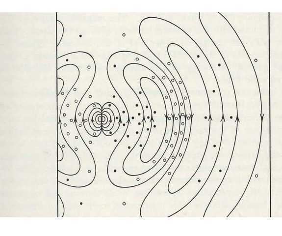
Fig. 1 – Electric and Magnetic Fields Near a Radiating Short Dipole Antenna

From the Es to the Em Field.

Fig. 1 (Ref. 5) shows the generation of the Em field from the Es field. The electric wave begins as a pure Es field close to the antenna; this is indicated by the flux lines between charges attached to the antenna.

But from the beginning, the Es field generates an H field shown by the dots in & out of the page. This H field in turn generates the closed-loop Em field by Maxwell’s equation $\nabla \times \bf H = \partial \bf D/\partial t$. As the field radiates away from the antenna the Es field diminishes while the Em field assumes predominance. For r > 1 wavelength the wave is essentially wholly Em and is isolated from further antenna Es field generation.

The E Field in Spherical Coordinates

In spherical coordinates $(r, \theta, \phi)$ , with $\theta$ the polar angle $0 < \theta < +\pi$ and $\phi$ the azimuth angle $0 < \phi < 2\pi,$ the dipole antenna stretches from $(d/2,-\pi)~ to~ (d/2,0)$. The combined $\bf E = \bf Es + \bf Em$ field has $r$ and $\theta$ components $E_r$ and $E_{\theta}$, with the $\phi$ component zero.

The antenna Induction Field

In the “near” or “induction” field, $E_r$ and $E_{\theta}$ fall off with distance r as $(1/r^3).$ The electric field of a quasi-stationary oscillating dipole at frequency $\omega$ can be expressed as

$\bf E_s = (1/4\pi) (1/r^3) [(3 \bf p \cdot \hat {\bf r})~\hat {\bf r} – \bf p]e^{j \omega t}$

where $\bf p$ is the dipole moment. $\bf E_s$ is then resolved into spherical $r$ and $\theta$ components and compared with $E_r$ and $E_{\theta}$ obtained above.

Es Field Amplitude Similar to that of a Low-frequency  Oscillating Dipole

Doing this comparison we see that the roll off with $1/r^3$ is the same for the quasi-stationary dIpole as for the antenna’s induction field. Thus, E accordingly behaves predominantly as an Es field; nearly exactly so at the antenna itself as $r \to 0$.

The Antenna Radiation Field

In the “far” or “radiation” field the only surviving E component is $E_{\theta}$, falling off as $1/ \lambda r$. Obviously, the E field at large distances is practically wholly Em. (The idea of electrons “flying thru the air” is picturesque but strictly metaphoric! So, no charges, no Es field).

There is an intermediate area where $E_r$ and $E_{\theta}$ coexist and roll off primarily as $1/r^2$ . At a distance $\lambda/r = 2\pi$ the Es and Em amplitudes are equal.

A Picture of the Evolving  Antenna Radiation Pattern

With the aid of fig. 1 the above presents a fascinating picture of the E fields at near, intermediate, and long distances from the antenna. The field very near the antenna is wholly Es but an H field is also immediately generated, by $\nabla \times \bf H = \epsilon_0 \partial \bf E_s/\partial t$ . As we go out in distance the H field produces an Em field by $\nabla \times \bf H = \epsilon_0 \partial \bf E_m/\partial t$.

Thus Es transitions into a mixed Es and Em field and then finally metamorphoses into a pure Em field, totally independent of the antenna current, traveling to the outreaches of space in closed loops.

Em and Es Fields at a Receiving Antenna

At the receiving end, the Em wave induces an equal and opposite Es field within the antenna, the latter generating a detectable voltage V per $V = \int \bf E_s \cdot \bf dl$ integrated over the antenna length.

Final Observations on Es and Em fields

It is sometimes asked, why be concerned with the existence of two kinds of electric fields when ignoring it can often fully account for available experimental data?

1.  It can identify the presence of charge distributions not otherwise identifiable. Since when is it not of interest that charges are formed?  Since when is it not the case that charges set up electric fields?  Dr.  Coulomb would be very surprised.
2. It can preclude uninformed statements such as “Kirchhoff was wrong”.
3.  It can correct the mistaken idea that “voltage is the line integral of the electric field” without qualifying that this applies to irrotational (i.e. Es) fields only.
4.  It can identify erroneous rationale even in sources of otherwise impeccable authority.  (I can give at least one example by PM if desired.)
5. Again, we are physicists so should gain as deep an understanding of physics as possible.  This should be our goal, not merely explaining limited test results based on inadequate test procedures and apparatus (e.g. see #1 above).

Summary

We see that the two kinds of the electric field, previously analyzed in other Insight blogs in electrostatic and quasi-static environments, exist in dynamic conditions as well. Awareness of this duality often yields vital information about the source and behavior of electric fields in many applications.

1. https://www.physicsforums.com/insights/a-new-interpretation-of-dr-walter-lewins-paradox/

2. https://www.physicsforums.com/insights/introduction-to-electric-vector-potential-and-its-applications/ including appended references

3. https://www.feynmanlectures.caltech.edu/II_23.html

4. H.H. Skilling, Fundamentals of Electric Waves, 2nd Edition, John A. Wiley & Sons.

5.  https://farside.ph.utexas.edu/teaching/em/lectures/node45.html