Intro to Data Structures for Programming

Introduction

In the first part of this series, I talked about some fundamental notions in the world of algorithms. Beyond the definition of an algorithm, we saw the criteria, ways to represent an algorithm, the importance of correctness, and elements of the classification and analysis of algorithms. It has also become evident that it is of crucial importance to have a well-designed and thoroughly tested algorithm, in order to achieve an optimal solution for our problem at hand.

But this is not the whole story regarding our preparation for an optimal solution to a problem. There is a second crucial component or better, “ingredient”, that goes hand-in-hand with an algorithm: the chosen data structure(s). Effective use of the principles of data structures boosts the efficiency of algorithms to solve problems like searching, sorting, etc. As Niklaus Wirth has stated it in the title of his 1976 book “Algorithms + Data Structures = Programs”$^{[1]}$. This points out the importance of a data structure in the procedure of developing an efficiently written program. Also, the two concepts on the left-hand side of the “equation” in this title, are inherently related. The famed algorithm designer Robert Tarjan was once quoted as saying that any problem can be solved in $O(n \log n)$ time with the right data structure.

In this first part of the second tutorial of this series of insights, I’ll talk about the main notions of data structures in general and then about some elementary Abstract Data Types (ADTs) and data structures. We’ll see arrays and linked lists and the abstract data types list and stack, some of their implementations, and some of their uses. The subject is really huge so my focus will be on giving as many crucial things as I can, in a first-things-first fashion. The reader is assumed to have sufficient familiarity with the topics presented in the first part and also some basic familiarity with at least one procedural programming language.

A few more things about the complexity and the analysis of algorithms

Before delving into data structures, it is important to say a few more things about the complexity and the analysis of algorithms.

Turing Machines

In the first tutorial, I said a few things about the analysis of algorithms. The theoretical study of algorithms and the classification in complexity classes use the Turing Machine$^{[2]}$ model. A Turing Machine (TM) is an abstract machine, defined by a mathematical model of computation. Very briefly, a TM consists of

– A tape divided into cells, one next to the other. Each cell is usually blank at the start and can be written with symbols from some finite alphabet including a special blank symbol. The tape is arbitrarily extendable to the left and to the right
– A head that can read and write symbols on the tape. With this head, the machine can perform three very basic operations
$\space\space\space\space$- Read the symbol on the square under the head
$\space\space\space\space$- Edit the symbol by writing a new symbol or erasing it
$\space\space\space\space$- Move the tape left or right by one square so that the machine can read and edit the symbol on a neighboring square
– A state register that stores the state of the Turing machine
– A finite table of instructions

A detailed description of how a TM operates, it’s the formal (mathematical) definition and the different kinds of TMs are subjects of Theoretical CS and they’re outside the scope of this tutorial. However, I highly recommend the reader to, at least, read the whole article in the resource given above if he/she doesn’t know about TMs.

What is of interest in our present discussion is that, despite its simplicity, a TM can simulate any computer algorithm. According to the Church – Turing thesis, TMs indeed capture the informal notion of effective methods in logic and mathematics and provide a precise definition of an algorithm.

The RAM model

A widely used model for the description and analysis of algorithms is the RAM (Random Access Machine) model which refers to computing machines, consisting of one general-purpose processor which cannot execute concurrent operations. Such a machine

– Has the necessary registers, an accumulator, and a sequence of storage locations with addresses 0, 1, 2, … which comprise its main memory
– It is able to perform arithmetic operations (+, -, *, /, mod), make decisions for branching (if type), based on the operators =, <, >, <=, >=, <> and read / write from / to memory.

Now, the primitive operations mentioned above have a time cost. There are two different approaches to measure this cost:

The first, called unit cost measure, assigns a constant (finite) cost to each operation, regardless of the length of the binary representation of its operands. The second, called logarithmic cost measure, assign a time cost that is proportional to the length of the binary representation of the operands for some specific operation. In most cases, we use the first approach unless there is an extensive number of operations performed on bit strings. But how do we use the RAM model for the analysis of algorithms?

As already mentioned, we mostly use the first approach above (unit cost measure). We also take into account the input size. The meaning of input size is different, depending on the problem at hand. If we have a sorting algorithm, for example, the input size is the number $n$ of the items to be sorted. For an algorithm that computes the Minimal Spanning Tree (MST) of a graph $G = (V, E)$, where $V$ is the set of vertices and $E$ is the set of edges of the graph – I’ll talk about graphs in the next part of this tutorial, the input size is $n = |V| + |E|$.

On the other hand, if the job of the algorithm is to perform an operation e.g. multiplication of two large integers then the input size is the total length (number of bits) of their binary representation and not the number “two”. So, time cost and space cost – in most cases we’re interested in time cost, of an algorithm for a certain input, is the number of primitive operations or steps performed and the number of memory locations needed respectively, for a RAM model implementation. The calculations are done in the following way:

(a) For every instruction regarding the assignment of a value or variable declaration for both logical and arithmetic operations, we charge constant time

(b) Repetition structures have time cost equal to the number of repetitions multiplied by the number of instructions performed in each repetition

(c) A simple type variable has constant space cost $O(1)$ while a k-elements array has time and space cost $O(k)$

In many cases, it is sufficient to locate the so-called, dominant operations, of the algorithm i.e. operations with a critical role regarding the behavior of the algorithm, so we focus our attention on them. As an important example, for sorting algorithms, the dominant operations are the comparisons and the interchange of elements between two positions of the input array. In order to calculate the time cost, we use the number of comparisons and interchanges that take place. I’ll give an example of analysis using the above procedure in the section of arrays.

Oftentimes, we may not be able to find a specific formula for the time or space cost or we may not be interested to do so. In these cases, we just deal with the rate of growth or order of growth of the function(s) that express the complexity of an algorithm, as I describe in the section “Analysis of algorithms” in the first part.

Also, there are cases in which, due to the presence of an inherent probability distribution, the running time of an algorithm may differ on different inputs of the same size. In these cases, we use probabilistic analysis$^{[3]}$. In some such cases, we can assume that the inputs conform to some known probability distribution and we’re averaging the running time over all possible inputs. But there are cases in which the probability distribution does not come from the inputs but from random choices made inside the algorithm.

In any case, the RAM model is an indispensable tool for every programmer as there is definitely a number of cases, where we need it.

Data Structures

What is a data structure?

Definition

A data structure is a way to store and organize data in order to facilitate access and modifications.

We’ll start our journey into the world of data structures at a low level: the representation of data inside a computer. The basic unit of data representation is a bit. The value of a bit can be one of two mutually exclusive values: 0 or 1. A number of combinations of the two values of a bit are used to represent data in a different manner, in different systems. Putting eight bits together forms a byte that can represent a character. One or more characters form a string. So, a string is a data structure that emerges through several layers of other data structures. We can make the representation of a string more efficient and easier for us to utilize, by wrapping it into another data structure that can take care of the intricacies and support a number of operations like finding the length of a string, joining two strings, etc.

Now, let’s see how the primitive data types of any programming language are represented at an internal level (memory).

Integers

An integer is the basic data type used for storing integer numbers. We use binary number$^{[4]}$ system to represent the non-negative integers. There are two methods commonly used for the representation of negative integer numbers in a binary system: one’s complement$^{[5]}$ and two’s complement$^{[6]}$.

Real numbers

The representation method used is floating-point notation$^{[7]}$.
We represent the mantissa and the exponent using the binary number system and one’s or two’s complement. So, finally, we have a “merged” binary number in memory.

Characters

There are various different codes to store data in character form like ASCII$^{[8]}$, BCD$^{[9]}$ and EBCDIC$^{[10]}$.

Now, every computer has a set of native data types. This means that it is capable of manipulating bit patterns as binary numbers at various locations. In most programming languages, primitive data types are mapped to the native data types of a computer but in some programming languages, new types are offered that essentially rely on a software implementation of hardware instructions that can interpret bit strings in the desired fashion and perform the operations needed.

Abstract Data Types

An Abstract Data Type (ADT) is a mathematical model of the data objects that make up a data type$^{[11]}$ and the functions that operate on these objects. It is a specification of the mathematical and logical properties of a data type or structure in general. This specification does not imply implementation details that are different according to the syntax of a specific programming language. On the other hand, the term data type, in a programming language, refers to the implementation of the mathematical model specified by an ADT. So, effectively, such a data type defines the internal representation of data in memory.

But why all the above discussion about data types and ADTs and what these have to do with data structures?

There is an open relationship among these three notions: A data type, as we saw above, is the implementation of an ADT i.e. of a specification about the relationship of specific data and the operations that can be performed on them and data structures, at the programming level, are essentially sets of variables of the same or different data types. Here, we also make an important distinction: ADTs vs. Data Structures. An ADT, as we already saw, is essentially a specification. So, effectively, ADTs are purely theoretical entities that we use in conjunction with abstract descriptions of algorithms (meaning not real implementations as programs). We can classify and evaluate data structures through them. On the other hand, a Data Structure is a realization of an ADT i.e. involves aspects of implementation.

Now, let’s get to the (higher) level of program design. As I mentioned at the beginning of this part, besides an efficient algorithm we also need an efficient way to store and organize our data. This means a proper ADT and a proper data structure at the programming level. Conceptually, we can model this way of storing and organizing data, as a set of (inter)connected nodes obeying a set of mathematical and/or logical properties and having a specific relation to each other, where each node represents a piece of data. Most importantly, we can perform a set of operations on these data in a flexible and efficient way. But what kind of operations are we able to perform?

Basic Operations on Data Structures

The basic operations we can perform on a data structure are:

– Access: Visiting each and every node of the data structure
– Insertion: Putting a new node in the data structure
– Deletion: Deleting a node from the data structure
– Search: Searching for the location of a specific node
– Sorting: Sorting according to some criteria
– Copying: Copy a data structure to another one
– Merge: Merging two data structures

There are some other operations as well, that I’ll present on a case-by-case basis. On this same basis, I’ll also present the operations pertaining to the ADTs that I’ll talk about.

We can categorize data structures using various criteria. One categorization is based on linearity i.e. there are linear and non-linear data structures. Another one is dynamic and static data structures. The first, allow updates and queries. The second, allow queries but no updates. There are also explicit and implicit data structures. The former use pointers (i.e. memory addresses) to link the elements and access them (e.g. a singly linked list, for which I’ll talk about later) and so they use additional space. In the latter, mathematical relationships support the retrieval of elements (e.g. an array representation of a heap).

There is also a number of other considerations for choosing the right data structure, like internal vs. external memory i.e. a data structure that performs well for data fitting in internal memory (RAM), may not be efficient for large amounts of data that need to be stored in external memory (e.g. disk). Another consideration is space vs. time, a frequent trade-off between time and space complexity.

Now, let’s see the most commonly used ADTs and data structures. The presentation of the operations performed by the relevant algorithms corresponds to the imperative programming paradigm. I highly recommend the reader check the resources at the end of the tutorial for more.

List

The list is an ADT that represents an ordered sequence of elements. Several real-world objects have the form of a list e.g. a “To do” list, the table of contents for a book, etc.  Lists are also of special importance to Computer Science. For example, within every computer system, files within a folder, applications running at a specific moment, bookmarks in a web browser, lines of code in a program, and many others are examples of the general idea of a list, equipped with various operations like search, create, insert, delete, find, first, next, etc.

Let L be a list of objects of some data type, x be an object of that type and p be of type position. The operations we can perform on L are:

– Insert(x, p, L) : Insert x at position p in list L, moving elements at p and following positions to the next higher position. If the list has no position p the result is undefined.

– Locate(x, L) : Returns the position of x on list L. If x does not appear then End(L) is returned.

– Retrieve(p, L) : Returns the element at position p on list L. The result is undefined if p = End(L) or if L has no position p.

– Delete(p, L) : Delete the element at position p of list L. The result is undefined if L has no position p or if p = End(L).

– Next(p, L) and Previous(p, L) : return the positions following and preceding position p on list L. If p is the last position on L, then Next(p, L) = End(L). Next is undefined if p is End(L). Previous is undefined if p is 1. Both functions are undefined if L has no position p.

– MakeNULL(L) : Causes L to become an empty list and returns position End(L).

– First(L) : Returns the first position on list L. In case L is empty returns End(L).

– PrintList(L) : Print the elements of L in the order of occurrence.

I should note that the operations found in the bibliography may slightly differ in number and names among different books. In any case, the main operations, expressed in a formal way, can be defined as above (see $^{[B1]}$).

We typically implement a list either as an array, if it is static, meaning that has a specific size, or as a linked list if its size is not known in advance. In the latter case we use dynamic memory allocation and pointers.

Array

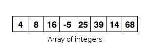
An array is an ordered collection of items, all of which are of the same type. Their elements can be anything that has a defined data type as also, other data structures. Arrays are linear data structures and also they are static. So, they occupy sequential memory locations. Also, in order to use them in programming, their size must be known in advance. Arrays can be one-dimensional or multi-dimensional.

Let’s see a simple example of an algorithm performing the operation of searching for a specific number, on a one-dimensional array of integers. Search in an array can be sequential or binary. Sequential search operates in a “brute force” fashion. It examines each and every element till it finds a match or till there are no more elements to examine.

Example 1

Problem

Given an array A of ten integers, write an algorithm that finds if a specific integer is present or not, and if present, it gives its position inside the array.

Solution

Note: The focus here is on sequential search, so for simplicity, we assume that the array is full i.e. we don’t fill it inside (i.e. as a part of) our algorithm. Also, the pseudocode is in a Pascal-like form. So, the array indexes start at 1.

Algorithm Sequential_Search

Data //i, k, num:INT
$\space\space\space\space\space\space\space\space$array A[10]:INT
$\space\space\space\space\space\space\space\space$found:BOOLEAN//

write “Give the number you’re looking for”
read num

i$\space\space$$\leftarrow$$\space\space$1
found$\space\space$$\leftarrow$$\space\space$false$\space\space\space\space\space\space\space\space\space\space\space\space$  !it will become true if we find the element we’re looking for
k$\space\space$$\leftarrow$$\space\space$0$\space\space\space\space\space\space\space\space\space\space\space\space\space\space\space\space\space\space\space\space\space\space\space$   !if we find the element this variable will hold its position in the array

while (i$\leq$ 10 AND found = false) do
$\space\space\space\space\space\space\space\space$if A[i] = num then
$\space\space\space\space\space\space\space\space\space\space\space\space\space\space\space\space$found $\space\space$$\leftarrow$$\space\space$true
$\space\space\space\space\space\space\space\space\space\space\space\space\space\space\space\space$k$\space\space$$\leftarrow$$\space\space$i
$\space\space\space\space\space\space\space\space$end_if
$\space\space\space\space\space\space\space\space$i$\space\space$$\leftarrow$$\space\space$i + 1
end_while

if (k = 0 OR found = false) then
$\space\space\space\space\space\space\space\space$write “Number is not found”
else
$\space\space\space\space\space\space\space\space$write “Number is found at position”, k
end_if

Binary search

Before getting to the topic of binary search, let me first say a few things about recursion.

Recursion

Recursion is a method of solving a problem by first solving smaller instances of this problem. In order to present this concept in a comprehensible way, I’ll utilize the notion of a function i.e. a series of steps that return some result, that calls itself either directly or indirectly through another function. We call such a function recursive.

Let’s say that we call such a function from our main program or from another function. A recursive function actually knows how to solve only the simplest case(s) of a problem, the so-called base case(s). So, if we call the function with a base case then it just returns some result. But if we call it a more complex problem, it divides the problem into two (conceptual) pieces: one that knows how to handle and one that it doesn’t.

In order for the recursion to be doable, the second piece must resemble our original problem albeit being simpler. As this new problem looks like the original one, the function calls a fresh copy of itself in order to work on the simpler (or smaller) problem, so here we have a recursive call. This is also called the recursion step. Also, at this step, the function returns (i.e. in programming terms we have a return statement), in order for the result to be combined with the portion of the problem for which the function knew how to handle and so a result will be formed to be given back to the original caller of the recursive function.

A very important point is that the recursion step executes while the original call to the function is still open. The recursion step may result in more such recursive calls because for each new subproblem it is called with, the function keeps dividing it into two pieces. In order for this process to terminate, the sequence of smaller problems formed by the calls of the recursive function to itself with a smaller problem each time must eventually converge on the base case. Reaching that point, the function recognizes the base case and a sequence of returns to previous copies of the function ensues all the way up the line until the original call of the function eventually returns the final result to the main program.

To illustrate all the above let’s see an example of a recursive function

Example 2

Problem

Write a recursive function which computes the factorial of a natural number $n$ $(n\leq 15)$

Solution

Before getting to the solution, a clarification first: we ask $n$ to be up to $15$ just for illustrational purposes as the focus is on the way that a recursive function works. For big $n$ values we just have to use the appropriate data type.

We define the factorial of a natural number  recursively as $n! = n\cdot (n – 1)!$ with $0! = 1$. So, we can write our recursive function as

function factorial (n:INT):INT

if n = 0 then
$\space\space\space\space\space\space\space\space$factorial$\space\space$$\leftarrow$$\space\space$ 1$\space\space\space\space\space\space\space\space\space\space\space\space\space\space\space\space\space\space\space\space\space\space\space\space\space\space\space\space\space\space$!initial condition (base case)
else
$\space\space\space\space\space\space\space\space$factorial$\space\space$$\leftarrow$$\space\space$ n$\cdot$factorial(n – 1)         !recursive step

The reader can see the base case i.e. the “simplest case” of our problem – as I state it in the above analysis of how a recursive function works, which the function knows how to solve and the “more complex” problem (recursive step in the above pseudocode) which does not know how to solve. So, the function calls a fresh copy of itself with a simpler version of the initial problem (n has become n – 1 now) and again, if n = 0, it is done otherwise it has an even simpler problem to solve – compared to the previous one, so it calls again a fresh copy of itself with a simpler problem (n has now become n – 2) till it finally reaches the base case.

In order to illustrate the use of our recursive function in a more clear way i.e. in the context of a program, I’ll present a program written in Pascal.

program factorial1 (input,output);
    var n,f: integer;
        ch: char;
    function factorial (k: integer): integer;
        begin
            if k = 0 then
                factorial:= 1
            else
                factorial:= k*factorial(k - 1);
        end;
    begin
        repeat
            repeat
                writeln('Give a positive integer up to 15:');
                readln(n);
            until (n >= 0) and (n <= 15);
            f:= factorial(n);
            writeln('The asked factorial is: ',n,'!= ',f);
            writeln('Do you want to run the program again? y/n ');
            readln(ch);
        until (ch = 'n') or (ch = 'N')
    end.

In the above program, we prompt the user to enter a value between 1 and 15 (line 14), and when he/she does so, we have the initial call to factorial function (line 17) with the argument of the number that the user entered. From there, the function factorial (lines 4 – 10) does its job (see, above, the pseudocode part of the solution) and when it’s done, it returns its result back to the caller, putting the returned value to the variable f. Then, the program displays the result to the user in a formatted way (line 18).

I have also added a way for the user to run the program all over again (lines 19 – 21) as a general useful feature for a simple program. I made my comments after the program in order to give a beginner a more complete explanation for the portions of the program that need it but as I will also explain in the third tutorial of this series, in programming, we have to use comments inside our programs in order to clear things up for anyone reading our program and where this is needed. Also, I didn’t put a line number in front of each line – as is the usual educational practice for outside-program explanations about the program, because the program has just a few lines.

Now, let’s get to our main topic of this section. Binary search is based on the principle of divide-and-conquer. In the first tutorial, I referred to a broad sense classification of algorithms, according to various criteria. One of them is the design pattern of an algorithm, which essentially determines the strategy that the algorithm will follow in order to solve a problem. Divide-and-conquer is such a strategy and, as its name implies, is based on dividing a problem into a small number of pieces and conquer i.e. solve each piece by applying divide-and-conquer recursively to it. Finally, it combines the pieces together and forms a global solution.

In the context of arrays, binary search works only in a sorted array and starts by comparing the target value to the middle element of the array. If they are equal it is done otherwise it checks if the target value is bigger or less than the middle element of the array – this works for both ascending and descending sorting order. So, it rules out one half of the array and continues through the other, by again comparing to the middle element of this sub-array and so on till it finds a match or there are no more elements to check.

Now, let’s see the same problem of Example 1 solved using binary search. We again assume that the array is filled with integers and also, now, sorted in ascending order.

Algorithm Binary_Search

Data //i, num, l, r, m:INT
$\space\space\space\space\space\space\space\space$array A[10]:INT//

write “Give the number you’re looking for”
read num

l$\space\space$$\leftarrow$$\space\space$1                          !initialize the holder for the left index
r$\space\space$$\leftarrow$$\space\space$10                        !initialize the holder for the right index
m$\space\space$$\leftarrow$$\space\space$(l + r) div 2     $\space$!assign the integer quotient of (l + r) by 2 to m

while (l$\leq$r AND A[m] <> num) do
$\space\space\space\space\space\space\space\space$if num $<$ A[m] then
$\space\space\space\space\space\space\space\space\space\space\space\space\space\space\space\space$r$\space\space$$\leftarrow$$\space\space$m – 1
$\space\space\space\space\space\space\space\space$else
$\space\space\space\space\space\space\space\space\space\space\space\space\space\space\space\space$l$\space\space$$\leftarrow$$\space\space$m + 1
$\space\space\space\space\space\space\space\space$end_if

$\space\space\space\space\space\space\space\space$m$\space\space$$\leftarrow$$\space\space$(l + r) div 2
end_while

$\space\space\space\space\space\space\space\space$if A[m] = num then
$\space\space\space\space\space\space\space\space\space\space\space\space\space\space\space\space$write “The number you gave is found at position”, m, “of the array”
$\space\space\space\space\space\space\space\space$else
$\space\space\space\space\space\space\space\space\space\space\space\space\space\space\space\space$write “Your number was not found in the array”
$\space\space\space\space\space\space\space\space$end_if

If we wanted to have the array filled by the user in the above example, we could use a repetition structure e.g.

write “Give the elements of the array”
for i from 1 to 10
$\space\space\space\space\space\space\space\space$read A[i]

The reader may have noticed that the above algorithm “Binary_Search” is not recursive. Well, every recursive function or subprogram can be also written in a non-recursive way i.e. using repetition structures. In the third tutorial of this insights series, we’ll see some main points of recursion vs. iteration.

Now, the way we perform simpler operations like accessing an element, inserting a new element, or deleting an element in an array, should be obvious to the reader. We now proceed to sort.

Sorting

In the first tutorial of this series, we saw that sorting is the operation of rearranging the elements of a list in some specified order. There are various different algorithms we can utilize in order to perform sorting. I also said a few things about the analysis of algorithms. Using the task of analysis, we can see the efficiency of an algorithm.

For sorting algorithms there are two classes according to their performance. It is the $O(n^2)$ class for the Bubble Sort$^{[12]}$, Insertion Sort$^{[13]}$, Selection Sort$^{[14]}$ and Shell Sort$^{[15]}$ and $O(n\log n)$ for the Heap Sort$^{[16]}$, Merge Sort$^{[17]}$ and Quick Sort$^{[18]}$. This classification refers to the original version of each algorithm.

Insertion sort, Heap Sort, Merge Sort and Quick Sort are all comparison sorts i.e. they determine the sorted order of an input array by comparing elements. In order to study the performance limitations of comparison sorts, we can use the decision-tree model$^{[19]}$. Using this model, we prove a lower bound of $\Omega(n\lg n)$ on the worst-case running time of any comparison sort on $n$ inputs.

We can beat this lower bound if we can find a way to gather information about the sorted order of the input by some other means than comparisons. Examples are the Counting Sort$^{[20]}$ algorithm and a related algorithm, Radix Sort$^{[21]}$, which can be used to extend the range of counting sort. Also, Bucket Sort$^{[22]}$ – which requires knowledge of the probabilistic distribution of numbers in the input array, can, for instance, sort $n$ real numbers uniformly distributed in the half-open interval $[0, 1)$ in average-case $O(n)$ time.

Also, various combinations and modifications per algorithm are used on a case-by-case basis, in order to achieve better performance.

Now, the reader may wonder why learn some time-expensive algorithms at all? The answer is that they are used for educational purposes and in practice, in cases where the nature of the problem allows for it.

For the purposes of this tutorial, I chose to present an example of the Bubble Sort algorithm, as is usually done in introductory CS and programming courses. Bubble Sort is good as a simple example of the process of sorting. Other than that, in practice, Bubble Sort under best-case conditions i.e. on an already sorted list can approach a constant $O(n)$ complexity but in the general case has an abysmal $O(n^2)$.

Also, it should be pointed out that although the Insertion, Selection, and Shell sorts also have $O(n^2)$ complexities, they are significantly more efficient than Bubble Sort. The reader is advised to have a thorough look at the topic of the analysis of algorithms if he/she has not already done so.

Example 3

Problem

Write an algorithm, that uses the Bubble Sort technique to sort an array A of ten integers, in ascending order and prints the sorted array.

Solution

Before getting into the pseudocode of the solution, a few more things about Bubble Sort.

This sorting technique has taken its name from the fact that the smaller values gradually “bubble” their way upward to the top of the array, something like air bubbles going their way up in the water, while the larger values sink to the bottom. Using this technique, we make several passes through the array. On each pass, successive pairs of elements are compared. If a pair is already in increasing order or if the values are equal, the values are left the way they are. If a pair is in decreasing order, its values get swapped in the array.

Algorithm Bubble_Sort

Data //i, pass, hold:INT
$\space\space\space\space\space\space\space\space$array A[10]:INT//

for pass from 1 to 9                    !controls number of passes
$\space\space\space\space\space\space\space\space$for i from 1 to 9                  !controls number of comparisons per pass
$\space\space\space\space\space\space\space\space\space\space\space\space\space\space\space\space$if A[i] > A[i + 1]               !if a swap is necessary it is performed in the next three lines
$\space\space\space\space\space\space\space\space\space\space\space\space\space\space\space\space\space\space\space\space\space\space\space\space$hold$\space\space$$\leftarrow$$\space\space$A[i]        !the variable hold temporarily stores one of the two values being swapped
$\space\space\space\space\space\space\space\space\space\space\space\space\space\space\space\space\space\space\space\space\space\space\space\space$A[i]$\space\space$$\leftarrow$$\space\space$A[i + 1]
$\space\space\space\space\space\space\space\space\space\space\space\space\space\space\space\space\space\space\space\space\space\space\space\space$A[i + 1]$\space\space$$\leftarrow$$\space\space$hold
$\space\space\space\space\space\space\space\space\space\space\space\space\space\space\space\space$end_if
$\space\space\space\space\space\space\space\space$end_for
end_for

write “Array elements in ascending order”

for i from 1 to 10
$\space\space\space\space\space\space\space\space$write A[i]

In the above algorithm, we use the variable hold to temporarily store one of the two values being swapped. Couldn’t we just perform the swap with only the two assignments A[i]$\space\space$$\leftarrow$$\space\space$ A[i + 1] and A[i + 1]$\space\space$$\leftarrow$$\space\space$A[i]?

The answer is no. I leave the “why” as an exercise to the reader, as this is a very essential concept for a beginner programmer.

Now, as I said in the section of the RAM model above, let’s see an example of an analysis of the Selection Sort algorithm using this model.

Example 4

Problem

Find the time complexity of the Selection Sort algorithm performing on an array of N integers, using the RAM model

Solution

First, we write the pseudocode for the Selection Sort algorithm:

Algorithm SelectionSort

Data //i, j, n, min, temp: INT
$\space\space\space\space\space\space\space\space$array A[n]: INT//

for i from 1 to n – 1
$\space\space\space\space\space\space\space\space$min$\space\space$$\leftarrow$$\space\space$ i

$\space\space\space\space\space\space\space\space$for j from i + 1 to n
$\space\space\space\space\space\space\space\space\space\space\space\space\space\space\space\space$if A[j] < A[min] then

$\space\space\space\space\space\space\space\space\space\space\space\space\space\space\space\space\space\space\space\space\space\space\space\space$min$\space\space$$\leftarrow$$\space\space$j
$\space\space\space\space\space\space\space\space\space\space\space\space\space\space\space\space$end_if

$\space\space\space\space\space\space\space\space\space\space\space\space\space\space\space\space$if min <> i then
$\space\space\space\space\space\space\space\space\space\space\space\space\space\space\space\space\space\space\space\space\space\space\space\space$temp$\space\space$$\leftarrow$$\space\space$A[i]
$\space\space\space\space\space\space\space\space\space\space\space\space\space\space\space\space\space\space\space\space\space\space\space\space$A[i]$\space\space$$\leftarrow$$\space\space$A[min]
$\space\space\space\space\space\space\space\space\space\space\space\space\space\space\space\space\space\space\space\space\space\space\space\space$A[min]$\space\space$$\leftarrow$$\space\space$temp
$\space\space\space\space\space\space\space\space\space\space\space\space\space\space\space\space$end_if
$\space\space\space\space\space\space\space\space$end_for
end_for

The algorithm divides the array into two parts: one sub-array of integers already sorted, which is built up from left to right at the front (left) of the initial array, and the sub-array of integers remaining to be sorted, that occupy the rest of the initial array. Initially, the sorted sub-array is empty and the unsorted sub-array is the entire input array. The algorithm proceeds by finding the smallest element in the unsorted sub-array. It then swaps it with the leftmost unsorted element (putting it in sorted order) and so, it moves the sub-array boundaries one element to the right.

Analysis of Selection Sort

As we saw in the section for the RAM model, the number of operations that an algorithm performs typically depends on the size, $n$, of its input. For sorting algorithms, $n$ is the number of elements in the array. We also saw that for sorting algorithms, the dominant operations are the comparisons and the interchange of elements between two positions of the input array.

In the above pseudocode we see that in order to sort $n$ elements, Selection Sort performs $n – 1$ passes (outer for-loop). Now, going to the inner for loop, on the first pass it performs $n – 1$ comparisons to find the minimum index (min), on the second pass it performs $n – 2$ comparisons, and so on till the last ($n – 1$) pass that performs one comparison.

So, if we add up the number of comparisons performed on each pass we get: $C(n) = 1 + 2 + … + (n – 1) = \frac{n(n – 1)}{2}$. Going to the second if, which checks for swapping, we easily see that it is executed at most $n$ times. So, if we assign a time cost $c1, c2, c3,\dots$ to each line of the pseudocode – lines excluded from the analysis can be easily identified, and taking each if statement as one instruction and starting from the first (outer) for loop up to the end, we multiply by the number of times their statements are executed and so get the equation $T(n) = (c3 + c4)\frac{n^2}{2} + (c1 + c2 – \frac{c3}{2} + \frac{c4}{2} + c5 + c6 + c7 + c8)n$, which gives the worst case time cost.

As previously said, oftentimes, we may not be able or we may not be interested in calculating the time cost in such detail. For the above calculation, we can take an asymptotic approximation from the dominant $\frac{n(n – 1)}{2}$ factor and it is $\frac{n^2}{2}$. We’re also not interested in $\frac{1}{2}$ in this case and finally, we have the worst time complexity of $O(n^2)$.

Returning to the basic operations we can perform on a data structure, copying an array B into another array A of the same size should now be straightforward to the reader: we use a repetition structure to run through the elements of both arrays and we assign the elements of B to A in an element-by-element fashion i.e. A[i]$\space\space$$\leftarrow$$\space\space$B[i].

Merging two sorted arrays is the last operation we’ll talk about in this section. This is an operation that copies the elements of both two initial arrays to a third array. Below, I’ll give the steps in order to merge two arrays in physical language with steps form. Writing the pseudocode from these steps should be a straightforward task, so I leave it as an exercise to the reader.

Example 5

Write the steps needed in order to merge two sorted arrays of integers A and B and store the resulting list of elements to the third array of integers C.

Solution

Note: Here, without loss of generality, we assume that both A and B as also C (where we’ll store our resulting list of elements) are / will be sorted in ascending order.

– Create array C to hold the resulting (merged) list of elements.
– Iterate over A and B
– Check current element of A
$\space\space\space\space\space\space\space\space$- If smaller than the current element of B store it to C.
$\space\space\space\space\space\space\space\space$- Else store the current element of B to C
– If there are elements left in A and / or B append them to C.

We saw the basic operations we can perform on an array. What are the advantages of using this data structure in programming? An advantage is that we have a collection of data items stored in a sequential manner. This guarantees very fast access to any element of an array, regardless of the array size. That’s why we call arrays “random access structures”. But what if we want to find a specific value inside an array?

This is the search operation we previously saw. This is a costly operation in general, although we can use techniques like sorting and binary search to improve performance in a remarkable way. Also, inserting or deleting an element are costly operations in general because they require the movement of elements. So, it depends on the case at hand if it is beneficial to use an array or not. Another important point is that we use arrays in order to implement various ADTs. This will become clear later in the tutorial.

Linked List

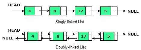
A linked list is a data structure that consists of a collection of nodes. Each node contains data and a pointer to the next node in the sequence. So, the order of the data elements is not given, in general, by their physical locations in memory.

What is a pointer? Pointers is an extremely important concept of programming languages having low-level features.
A pointer is a variable that stores a memory address. Normally, a variable directly contains a specific value. A pointer, on the other hand, contains an address of a variable that contains a specific value. So, a pointer indirectly references a value.

A linked list can be

•  Singly-linked : The elements are linked by a single pointer. This structure allows the list to be traversed from its first element to its last.
•  Doubly-linked : The elements are linked by two-pointers instead of one. This structure allows the list to be traversed both forward and backward.
•  Circular : In this type of linked list the last element is linked to the first instead of being set to NULL.  This structure allows the list to be traversed in a circular fashion.

Linked lists maintain collections of data, similar to what we often use arrays for. The primary advantage of linked lists over arrays is that linked lists can grow and shrink in size during their lifetime. So, we don’t need to know their maximum size in advance. A second advantage is a flexibility that linked lists provide in allowing an efficient rearrangement of items. But this is at the expense of quick access to any item on the list.

Applications

Some important applications of linked lists are:

• Memory Management : This is an important role of operating systems. An operating system must decide how to allocate and reclaim storage for processes running on the system. A linked list can be used to keep track of portions of memory that are available for allocation.
• Linked allocation of files : Using this type of file allocation we eliminate external fragmentation on a disk but it is good only for sequential access. There is a pointer from each block of a file to the next.

Linked lists are also used to implement ADTs like stacks, queues, hash tables, and graphs among others.

Before delving into the specifics of the various types of linked lists, one note is in order: when studying the operations, the reader should first experiment and see for him/herself how the operations are carried out in a visual way i.e. by using a sketch of the list in question with just pen and paper. This will help very much in order to understand how the various operations are coded.

Singly-linked List

We can define a singly-linked list, in a formal way, as follows

type
$\space\space\space\space\space\space\space\space$celltype = record
$\space\space\space\space\space\space\space\space$element: elementtype;
$\space\space\space\space\space\space\space\space$next: (pointer) celltype
$\space\space\space\space\space\space\space\space$end;
LIST = (pointer) celltype;

This is a definition in pseudo-Pascal. The same definition in pseudo-C – well… “pseudo” here refers only to “elementtype”; putting an acceptable data type in C, gives us real code) is

typedef struct celltype {

$\space\space\space\space\space\space\space\space$elementtype element;
$\space\space\space\space\space\space\space\space$struct celltype * next;
} cell;

where we define a single node (“cell”). Then we can define a variable of the “cell” type like

cell * head = NULL;

, and give a value to “head”, as also, a pointer to the next node and so on. If we give the pointer a NULL value i.e. head $\space\space$$\rightarrow$$\space\space$next = NULL; we’re finishing the population of the list.

At this point, it is more interesting to use real code in order to show some of the operations we can perform on a singly-linked list. C programming language provides primitive operations that allow linked lists to be implemented directly. We’ll see the operations of adding a node at the beginning and at the end of a linked list, deleting a node, and searching for a particular value. I’ll just give the necessary definitions and the functions implementing the aforementioned operations, so the reader can get a general idea. Again, it is assumed that the reader has a knowledge of the basic syntax and constructs of a procedural language like Pascal or C.

We first define a member of our data structure and create it and then go on with the operations. Here we assume that we have data of type int.

typedef struct node {
    int data;
    struct node *next;
};
struct node *head;
head = NULL;

/* Inserts the value in front of the list.
Takes the head pointer and the value to be inserted.
Returns the new head pointer value */

struct node *insertFront(struct node *ref,int val) {
    struct node *p;
    p = (struct node *) malloc(sizeof(struct node));         //allocate the necessary memory
    p->data = val;
    p->next = ref;
    return p;
}

/* Inserts the value at the end of the list (as last element).
Takes the head pointer and the value to be inserted (NULL if list is empty).
Returns the new head pointer value */

struct node *insertEnd(struct node *ref,int val) {
    struct node *p,*q;
    p = (struct node *) malloc(sizeof(struct node));
    p->data = val;
    p->next = NULL;

    if (ref == NULL) return p;         //if list passed is empty then return just the node created
    q = ref;

    while (q->next != NULL)
    q = q->next; /* find the last element */
    q -> next = p;
    return ref;
}

/* Deletes a node from the list.
Takes the head pointer and the element to be deleted.
Returns the new head pointer value */

struct node *delete(struct node *ref, int val) {
    struct node *p, *q;
    p = ref;
    q = p;

    while(p!=NULL) {

        if (p->data == val) {
            if (p == ref) ref = p->next;
            else q->next = p->next;
            p->next = NULL;
            free(p);
            return ref;
        }
        else {
                q = p;
                p = p->next;
        }
    }
        return ref;
}

/* Searches the list for a specific value.
Takes the head pointer and the value to be searched.
Returns the node with the asked value if found otherwise returns NULL */

struct node *search (struct node *ref, int val) {
    struct node *p;
    p = ref;

    while (p != NULL){

        if (p->data == val) return p;
        p = p->next;
    }
    return p;
}

Now, we can call any of the above operations from our main program.

The above operations are not all the operations we can perform on a singly-linked list but I think that they give the general idea and enough motivation to the reader to think about / search for the rest.

Doubly-linked List

Compared to a singly-linked list, a doubly-linked list contains an extra pointer typically called “previous”. This gives to a doubly-linked list the advantages of traversing it both forward and backward, easily inserting a node before a given node, and more efficient delete operations. As a disadvantage, extra space is required for each node due to the extra pointer. Also, the “previous” pointer must be maintained in all operations.

We can define the doubly-linked list structure as shown below. Here we assume that we have data of type int.

struct dlNode {
    int data;
    struct dlNode * next;
    struct dlNode * prev;
}

The operations we can perform on a doubly-linked list are the same as on a singly-linked list but we have to always take care of the second pointer (pointing to the previous node of a certain node).

Now, let’s see how we perform addition of a node after a given node.

void insertAfter(struct dlNode *pre, int newData) {

    if (pre == NULL) { //check if the pre node is NULL
        printf("Node given cannot be NULL");
        return;
    }

    struct dlNode *new = (struct dlNode *)malloc(sizeof(struct dlNode)); //allocate new node
    new->data = newData; //put data
    new->next = pre->next; //make next of new node as next of pre
    pre->next = new; //make the next of pre as new
    new->prev = pre; //make pre as previous of new

    if (new->next != NULL)
        new->next->prev = new; // if next of new is not NULL change previous of new's next node
}

After giving the manipulation of the extra pointer in the above example operation, I encourage the reader to write by him/herself the rest of the operations, with the help of the respective operations on a singly-linked list.

We can create a memory-efficient version of a doubly-linked list with only one space for the address field of each node. This is called XOR Linked List$^{[23]}$, as it uses the bitwise XOR operation to save space for one address.

Circular Linked List

A circular linked list (a.k.a circularly-linked list) can be either singly linked or doubly linked. In order to traverse a circularly linked list, we begin at any node and follow the list until we return to the original node.

Advantages of a circular linked list are

– Depending on the nature of the problem at hand there are problems that lend themselves to a solution using a circular linked list.
– The entire list can be traversed starting from any node
– When implementing a circular linked list we have to care for a fewer number of special cases.

Some disadvantages are

– If we need to perform a search e.g. when we want to insert a node at the start of a list and depending on the implementation, if this needs a search for the last node, the search could be expensive.
– As there is no NULL pointer at the start or end, looping through nodes is harder.

In order to make an improvement, we can set a pointer only to the last node as then the start node will be pointed to by the last node.

Some usual operations we perform on a circular linked list are

– Insertion (at the beginning, at the end, or at a specific location in the list)
– Deletion (from the beginning, from the end, or a specific node)
– Display

Let’s create a new node for a circular linked list and code the display operation.

typedef struct circLLNode {
    int data;
    struct circLLNode *next;
}node;

node *front = NULL, *rear = NULL, *temp; //make the front and rear nodes NULL

void create() {
    node *new;
    new = (node*)malloc(sizeof(node));
    // reader is encouraged to enter here the C code to input data for the node
    new->next = NULL;

    if (rear == NULL)
        front = rear = new;
    else {
            rear->next = new;
            rear = new;
    }

    rear->next = front;
}

void display() {
    temp = front;

    if(front == NULL)
        printf("Empty List");
    else {
            for (;temp != rear;temp = temp->next)
            // reader is encouraged to enter the C code for displaying nodes
    }
}

The reader is encouraged to create a full C program that utilizes the above struct definition and functions as well as insert the code needed inside the above functions, as described in the comments.

Before going on to an important application of arrays and linked lists, I should mention that we can implement a linked list without using pointers. The basic idea is that we can split the two parts of a node of a linked list – data and next, and store them in two arrays for the data items and next nodes (for all nodes) respectively. In this way, the contents of the second array are integers denoting the next data item in the first array.

Now, one important application of arrays and linked lists is polynomials.

Polynomials

A polynomial, $P(x)$, is an expression of the form $ax^n + bx^{n-1} + \cdots + jx + k$ where $a, b, c,\dots, k$ are real numbers, $x$ is the variable and $n$ is a non-negative integer. The number $n$ is the degree of the polynomial. We can represent a polynomial as a list of nodes, where each node consists of a coefficient and an exponent. In order to implement such an ADT as a data structure there are some important points:

• The sign of each coefficient and exponent is stored within the coefficient and exponent itself
• We can add terms only if their exponents are equal
• Storage of each term in the polynomial must be done in ascending / descending order of their exponent

We can represent and do various operations on polynomials using arrays or linked lists. Let’s first see how we represent and do addition for two polynomials using arrays. We first define a structure for each term of the polynomials. Then we can use an array of such terms to represent each polynomial, take the polynomial terms as input from the user, store them into the corresponding arrays and do the operations we need. Below is a simple C program to do these steps which illustrates the basic ideas for polynomials of up to 10 terms. It would be very useful for the reader to add checks and other details if needed.

#include<stdio.h>

struct pol {
    float coeff;         //coefficient of type float
    int exp;             //exponent of type int
};

struct pol a[10], b[10], c[10];

int main() {
    int i;
    int deg1, deg2;      //degree of each polynomial
    int k = 0, l = 0, m = 0;
 
 
printf("Enter the degree of the first polynomial:");
scanf("%d",&deg1);
 
for(i = 0;i <= deg1;i++) {                                
    printf("\nEnter the coefficient of x^%d :", i);
    scanf("%f",&a[i].coeff);            
    
    a[k++].exp = i;      
}

printf("\nEnter the degree of the second polynomial:");
scanf("%d",&deg2);
 
for(i = 0;i <= deg2;i++) { 
    printf("\nEnter the coefficient of x^%d :",i);
    scanf("%f",&b[i].coeff);
	   
    b[l++].exp = i;
}

/* We can print the polynomials as a visual aid to the user */

printf("\nPolynomial1 = %.1f",a[0].coeff);
  
for(i = 1;i <= deg1;i++) {
    printf("+ %.1fx^%d",a[i].coeff,a[i].exp);
}    
  
printf("\nPolynomial2 = %.1f",b[0].coeff);

for(i = 1;i <= deg2;i++) {
    printf("+ %.1fx^%d",b[i].coeff,b[i].exp);
}

/* Polynomial addition */	

if(deg1 > deg2) {
    for(i = 0;i <= deg2;i++) {
        c[m].coeff = a[i].coeff + b[i].coeff;
	c[m].exp = a[i].exp;
	m++;
    }
		  
    for(i = deg2+1;i <= deg1;i++) {
	c[m].coeff = a[i].coeff;
	c[m].exp = a[i].exp;
	m++;
    } 
} 
else {
       for(i = 0;i <= deg1;i++) {
           c[m].coeff = a[i].coeff + b[i].coeff;
           c[m].exp = a[i].exp;
           m++;
       }
    
       for(i = deg1+1;i <= deg2;i++) {
           c[m].coeff = b[i].coeff;
           c[m].exp = b[i].exp;
           m++;
       }
     }
  
printf("\nSum  = %.1f",c[0].coeff);
    for(i = 1;i < m;i++) {
        printf("+ %.1fx^%d",c[i].coeff,c[i].exp);
    }	 
 
return 0;

}

Now, in order to develop a program with the same functionality using the linked list concept instead of arrays, we can define an appropriate structure and use the concept of pointers in order to store the various terms of each polynomial. Then we can write some functions for the various operations we need to perform (create, display, add) and call them from our main program. We have to be careful in the allocation of memory. For instance, allocating more memory for extra terms of the polynomial only when needed. I strongly encourage the reader to develop such a program, using the relevant parts of what I have presented in this tutorial so far.

Stack

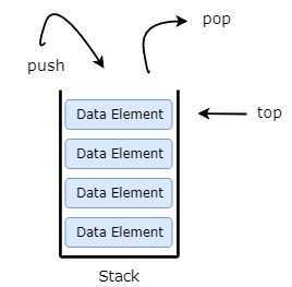
Stack is an ADT that serves as a collection of elements with the following operations defined on it:

– create            Create a new, empty stack
– empty             Return true if the stack is empty
– push              Insert a new element
– top               Return the element most recently inserted, if the stack is not empty
– pop               Remove the element most recently inserted if the stack is not empty

This is a specification referring to an ideal, unbounded stack.

A common way to depict a stack in order to understand its operations is using a pile of dishes: we put the first dish and then the second on top of the first, the third on top of the second, and so on. So, we initially have an empty stack and we use the push operation to add dishes. If we want to take a dish from the pile we take (pop) the current top one which is the last so far. So, the stack is a LIFO (Last In First Out) queue.

In order to describe the above specification in a formal mathematical way, so the reader can get an idea of how we formally define an ADT, I chose the commonly used approach (for the definition of ADTs) of expressing the semantics of the operations by relating them to each other. The other approach is to refer explicitly to the data contents of the stack.

Let $S$ be a set and $s_0$ in $S$ a distinguished state, where $s_0$ denotes the empty stack. Starting from the empty stack and performing finite sequences of “push” and “pop” operations, we obtain the set of stack states denoted by $S$. We can represent the stack operations with the following functions:

create: $\rightarrow$$\space\space S$
empty: $S\space\space\rightarrow\space\space$ {true, false}
push: $S\times X\space\space\rightarrow\space\space S$
top: $S – \{s_0\}\space\space\rightarrow\space\space X$
pop: $S – \{s_0\}\space\space\rightarrow\space\space S$

The semantics of the stack operations is specified by the following axioms

for all $s$ in $S$, for all $x$ in $X$, where $x$ is an element in the domain $X$ (data type):

1. create = $s_0$                       Produces a stack in the $s_0$ state
2. empty($s_0$) = true                  The (distinguished) $s_0$ state is empty
3. empty(push($s$, $x$)) = false         After an element has been inserted the stack is not empty
4. top(push($s$, $x$)) = $x$               The most recently inserted element is on the top of the stack
5. pop(push($s$, $x$)) = $s$               The inverse of “push” is “pop”

As noted above, this is a specification for the ADT stack but any real implementation can’t be unbounded like this.

So, a specific implementation imposes some bound on the size i.e. depth of a stack. Also, the way we’ll implement the stack ADT will define a particular data structure. We can implement the stack – according to our needs, either using an array which is of fixed length and the bound is on the maximum size of the array that we have at our disposal or using a linked list that does not have a fixed size – it can grow or shrink at execution time and the bound is on the size of the available memory.

In both cases, we have a data structure derived from a stack ADT but although the available operations on data are the same, these two data structures are quite different regarding their flexibility and their size.

For a fixed-length stack we have to add one more function to the above list of functions of the stack ADT. This function will check if the stack is full or not, so we can write it as:  “full: $\space\space S\space\space\rightarrow\space\space${true, false}”. In order to specify the behavior of this last function, we need another (internal) one, which measures the stack depth i.e. the number of elements currently in the stack. We can write this function as:  “depth: $\space\space S\space\space\rightarrow\space\space${0, 1, 2, … , m}”. Now, the axioms for specifying the stack semantics are

for all $s$ in $S$, for all $x$ in $X$:

create = $s_0$
empty($s_0$) = true
not full($s$)$\space\space\implies\space\space$ empty(push($s$, $x$)) = false
depth($s_0$) = $0$
not empty($s$)$\space\space\implies\space\space$depth(pop($s$)) = depth($s$) $- 1$
not full($s$)$\space\space\implies\space\space$depth(push($s$, $x$)) = depth($s$) $+ 1$
full($s$) = (depth($s$) = $m$)
not full($s$)$\space\space\implies\space\space$
$\space\space\space\space\space\space\space\space$top(push($s$, $x$)) = $x$
$\space\space\space\space\space\space\space\space$pop(push($s$, $x$)) = $s$

Now, let’s see an implementation of a fixed-length stack in Pascal.

const maxlen =    ;  (* value left blank as max length of the stack is defined by the user *)
type elemtp  =    ;  (* value left blank as stack elements type is defined by the user *)
    stack = record   (* we define stack as record which is a structured data type in Pascal *)
              arr: array[1 .. maxlen] of elemtp;
              dep:0 .. maxlen;    (* Holds the current depth of the stack *)
            end;

procedure create(var s: stack);
begin 
    s.dep := 0 
end;

function empty(s: stack): boolean;
begin 
    return (s.dep = 0) 
end;

function full(s: stack): boolean;
begin 
    return (s.dep = maxlen) 
end;

procedure push(var s: stack; x: elemtp);   
begin s.dep := s.dep + 1;
      s.arr[s.dep] := x
end;

function top(s: stack): elemtp;
begin
    return(s.arr[s.dep])
end;

procedure pop(var s: stack);
begin
    s.dep :=  s.dep - 1
end;

Now, two comments for the above implementation are in order. First, a structured data type is a compound data type that the user defines for grouping simple data types or other compound data types. Second, there is an assumption that the user checks that the stack is not full before calling push and that it is not empty before calling top or pop. Couldn’t we write these procedures in a way that eliminates this need? We could write them in a way that returns some error message to the caller but in this case, a further argument for each of the above procedures would be in order and this would lead to implementations that correspond to different ADTs than the ones discussed.

Applications

We use stacks in expression evaluation (prefix, postfix, and infix notation) e.g. in compilers as also, for the conversion from one of the previous forms of expressions to another. Many compilers use stacks for parsing the syntax of expressions, matching braces, program blocks, etc. Stacks can also keep information about active functions in a program and help in memory management. Backtracking of a path is also a concept in which the use of a stack can be useful.

Evaluation of arithmetic expressions

Let’s see some things about the evaluation of arithmetic expressions. More specifically we’ll see an algorithm that converts an infix expression to postfix notation and then an algorithm that evaluates a postfix expression. Let’s first see a few things about infix and postfix expressions.

Assume that the set of all permissible arithmetic expressions with parentheses consists of non-negative arguments (operands) and the arithmetic operators $+, -, *, /$. We can define an infix expression recursively as:

– A variable denoted by a letter $(A,\dots, Z)$ or a non-negative integer is an infix expression.
– If $A$ and $B$ are infix expressions then $(A+B)$, $(A-B)$, $(A\cdot B)$ and $(A/B)$ are also infix expressions.

This definition always presupposes the use of parentheses. However, in practice, this is not common. So, an expression like $(A+B)\cdot C$, is a valid infix expression like the normal $((A+B)\cdot C)$ which is consistent with the definition. This way, we avoid having too many parentheses in an expression.

The evaluation of such an infix expression is taking place according to the operator’s precedence. For doing this, we have to traverse the expression a number of times in order (each time) to locate the operators with higher precedence.  We can avoid this by converting the infix expression into postfix or prefix notation which has an easier evaluation.

The postfix notation of an expression (a.k.a reverse Polish notation$^{[24]}$) was invented by the Polish logician J.Lukasiewicz in 1924, is a notation in which the operators follow their operands. It has the advantage that its evaluation requires just one pass.

For the first algorithm, we’ll use a stack for storing operators and an array of characters for storing the postfix expression. We assume that the algorithm reads the infix expression from the file “input”. Both algorithms are in a pseudo-Pascal dialect.  “!” denotes comments.

while not eof(input) do
$\space\space\space\space\space\space\space\space$read(input, character)

$\space\space\space\space\space\space\space\space$if (character is operand) then
$\space\space\space\space\space\space\space\space\space\space\space\space\space\space\space\space$add character to postfix expression
$\space\space\space\space\space\space\space\space$else
$\space\space\space\space\space\space\space\space$if (character = ‘(‘) then
$\space\space\space\space\space\space\space\space\space\space\space\space\space\space\space\space$push (character, operators_stack)
$\space\space\space\space\space\space\space\space$else
$\space\space\space\space\space\space\space\space$if (character = ‘)’) then
$\space\space\space\space\space\space\space\space\space\space\space\space\space\space\space\space$while (top <> ‘(‘) do
$\space\space\space\space\space\space\space\space\space\space\space\space\space\space\space\space\space\space\space\space\space\space\space\space$pop(operator, operators_stack)
$\space\space\space\space\space\space\space\space\space\space\space\space\space\space\space\space\space\space\space\space\space\space\space\space$add the operator to the postfix expression
$\space\space\space\space\space\space\space\space\space\space\space\space\space\space\space\space$pop(operator, operators_stack)
$\space\space\space\space\space\space\space\space$else                                                           !character is operator
$\space\space\space\space\space\space\space\space$if not empty(operators_stack) then
$\space\space\space\space\space\space\space\space\space\space\space\space\space\space\space\space$while (precedence(character) $\leq$ precedence(top))
$\space\space\space\space\space\space\space\space\space\space\space\space\space\space\space\space\space\space\space\space\space\space\space\space$pop(operator, operators_stack)
$\space\space\space\space\space\space\space\space\space\space\space\space\space\space\space\space\space\space\space\space\space\space\space\space$add the operator to the postfix expression
$\space\space\space\space\space\space\space\space$push(character, operators_stack)

empty operators_stack into the postfix expression

The algorithm for the evaluation of a postfix expression follows

i$\space\space\leftarrow\space\space$1
character$\space\space\leftarrow\space\space$expression[1]                 !the postfix expression is stored into the string “expression”

while (character <> blank_char) do
$\space\space\space\space\space\space\space\space$if (character is number) then
$\space\space\space\space\space\space\space\space\space\space\space\space\space\space\space\space$push(number, variables_stack)      !a stack of variables is used globally as an auxiliary structure
$\space\space\space\space\space\space\space\space$else                                         !character is an operator
$\space\space\space\space\space\space\space\space\space\space\space\space\space\space\space\space$pop(number2, variables_stack)
$\space\space\space\space\space\space\space\space\space\space\space\space\space\space\space\space$pop(number1, variables_stack)
$\space\space\space\space\space\space\space\space\space\space\space\space\space\space\space\space$res $\space\space\leftarrow\space\space$number1 <operator> number2  !compute result
$\space\space\space\space\space\space\space\space\space\space\space\space\space\space\space\space$push(res, variables_stack)

$\space\space\space\space\space\space\space\space$if (i < postfix_expression_length) then
$\space\space\space\space\space\space\space\space$i$\space\space\leftarrow\space\space$i + 1
character$\space\space\leftarrow\space\space$expression[i]
$\space\space\space\space\space\space\space\space$else
$\space\space\space\space\space\space\space\space\space\space\space\space\space\space\space\space$character$\space\space\leftarrow\space\space$blank_char

pop(res, variables_stack)

In the next part, I’ll talk about Queues, Trees, Sets, and Graphs.

Bibliography

$^{[B1]}$ Alfred V. Aho, Jeffrey D. Ullman, John E. Hopcroft “Data Structures and Algorithms” First Edition, Pearson 1983

Robert Sedgewick “Algorithms in C, Parts 1 – 4: Fundamentals, Data Structures, Sorting, Searching” Third Edition, Addison-Wesley Professional 1997

Thomas H. Cormen, Charles E. Leiserson, Ronald L. Rivest, Clifford Stein “Introduction to Algorithms” Third Edition, The MIT Press 2009

Personal CS notes

Resources

$^{[1]}$ Niklaus Wirth “Algorithms + Data Structures = Programs” First Edition, Prentice Hall 1976
$^{[2]}$https://en.wikipedia.org/wiki/Turing_machine
$^{[3]}$https://en.wikipedia.org/wiki/Probabilistic_analysis_of_algorithms
$^{[4]}$https://en.wikipedia.org/wiki/Binary_number
$^{[5]}$https://en.wikipedia.org/wiki/Ones%27_complement
$^{[6]}$https://en.wikipedia.org/wiki/Two%27s_complement
$^{[7]}$https://en.wikipedia.org/wiki/Floating-point_arithmetic
$^{[8]}$https://en.wikipedia.org/wiki/ASCII
$^{[9]}$https://en.wikipedia.org/wiki/Binary-coded_decimal
$^{[10]}$https://en.wikipedia.org/wiki/EBCDIC
$^{[11]}$https://en.wikipedia.org/wiki/Data_type
$^{[12]}$https://en.wikipedia.org/wiki/Bubble_sort
$^{[13]}$https://en.wikipedia.org/wiki/Insertion_sort
$^{[14]}$https://en.wikipedia.org/wiki/Selection_sort
$^{[15]}$https://en.wikipedia.org/wiki/Shellsort
$^{[16]}$https://en.wikipedia.org/wiki/Heapsort
$^{[17]}$https://en.wikipedia.org/wiki/Merge_sort
$^{[18]}$https://en.wikipedia.org/wiki/Quicksort
$^{[19]}$https://en.wikipedia.org/wiki/Decision_tree_model
$^{[20]}$https://en.wikipedia.org/wiki/Counting_sort
$^{[21]}$https://en.wikipedia.org/wiki/Radix_sort
$^{[22]}$https://en.wikipedia.org/wiki/Bucket_sort
$^{[23]}$https://en.wikipedia.org/wiki/XOR_linked_list
$^{[24]}$https://en.wikipedia.org/wiki/Reverse_Polish_notation

Recommended Bibliography

M. H. Alsuwaiyel “Algorithms: Design Techniques and Analysis” Revised Edition, WSPC 2016

Peter Brass “Advanced Data Structures” First Edition, Cambridge University Press 2008