What Exactly is Dirac’s Delta Function?

Introduction: “Convenient Notation”

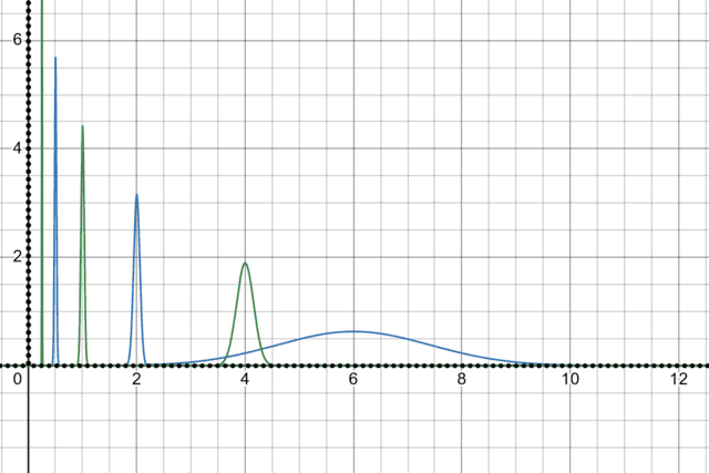
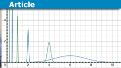
Approaching a Dirac delta function

In Dirac’s Principles of Quantum Mechanics published in 1930 he introduced a “convenient notation” he referred  to as a “delta function” which he treated as a continuum analog to the discrete Kronecker delta.  The Kronecker delta is simply the indexed components of the identity operator in matrix algebra:
$$\delta^j_k =\left\{\begin{array}{lcl}1&\text{ if } & j=k\\0&\text{ if }&j\ne k\end{array}\right.$$

The key utility of the Kronecker delta is its occurrence in summations:
$$a_k =\sum_{j=1}^N a_j \delta ^j_k$$

Similarly Dirac’s delta function is principally defined as it occurs in integrals:
$$f(y) = \int_{-\infty}^{\infty} f(x)\delta(x-y)dx .$$

Viewed another way the delta function allows you to evaluate the function at zero (and, via translations, elsewhere) by integrating:
$$f(0)= \int_{-\infty}^\infty f(x)\delta(x)dx$$
The problem is that no such function exists, as such, in the space of real functions.  The delta “function” is not, in fact, a function which is why Dirac referred to it as “convenient notation”.

This begs the question, “So what does this convenient notation represent?”  For the mathematician this means “Where’s the rigor?” and for the physicist it means “Will using this give me well defined predictions?”  This article points to some of the mathematical contexts in which Dirac’s convenient notation has been given proper mathematical meaning.

Riemann-Stieltjes integrals

We can formally define the Riemann-Stieltjes (R-S) Integral:
$$\int_a^b f(x) d g(x)$$
for well behaved real functions $f$ and $g$ in the same way we defined our Riemann integrals, as limits of (modified) Riemann sums.  Where $g$ is differentiable we can also prove integration by parts holds and express those R-S integrals as simple Riemann Integrals:
$$\int_a^b f(x) d g(x) = \left. f(x)g(x)\right\rvert_a^b -\int_a^b g(x)df(x) = \left. f(x)g(x)\right\rvert_a^b -\int_a^b f'(x)g(x)dx,$$
This is valid even when the derivative of $g$ is problematic in the interval of integration.
Of course identities are two way streets and we rewrite apparent Riemann integrals as well defined R-S integrals.

This is an improvement because Reimann-Stieltjes integrals have a broader domain of application.

The Dirac delta function as the “derivative” of the Heaviside step function

Consider the function $\Theta$ such that:
$$\Theta(x) = \left\{ \begin{array}{rcl} 1 & \text{if} & x\ge 0\\ 0 & \text{if} & x<0 \end{array} \right..$$
This is the Heaviside step function which is also denoted $H(x)$ in many texts.

Now consider the R-S integral:
$$I= \int_a^b f(x) d \Theta(x)\quad  a,b \ne 0.$$
Careful evaluation of the limit of the modified Riemann sum will yield zero if $0$ is outside the open interval $(a,b)$.  But for $a<0<b$ we get $I=f(0)$.  We can of course translate the step function $\Theta(x)\mapsto \Theta(x-c)$ to evaluate and any real value $c$:

$$f(c)=\int_a^b f(x)d\Theta(x-c)$$

We thus get the exact same behavior as Dirac’s “convenient notation” and we can use this as the definition of that notation:
$$\int_a^b f(x)\delta(x) dx \equiv \int_a^b f(x) d\Theta(x) .$$
Hence we often speak of the Dirac delta function as the “derivative” of the Heaviside step function.

The use of R-S integrals does not however deal directly with other equally convenient notations.  We can for example consider “derivatives” of Dirac’s delta function $\delta^{(n)}$ which have the defining property of evaluating the n-th derivative (with sign changes) of a function:
$$\int_{-\infty}^\infty f(x)\delta^{(n)}(x)dx \equiv (-1)^n f^{(n)}(0).$$

One can obtain this result by repeatedly applying integration by parts to peel off the formal derivatives of $\delta$ until one has a valid Riemann-Stieltjes integral.  This suggests we can extend the definition, say Extended Riemann-Stieltjes Integrals. However, this approach has now been supplanted with the more general Lebesgue integration.  Dirac’s delta function is considered (notation for) a distribution.  Specifically it is (and its derivatives are) expressed in terms of the Radon-Nikodym derivative(s) of the measure defined by the Heaviside step function.

There is a more operational approach to understanding Dirac’s delta function in terms of how it is actually being used.

Vectors, dual vectors, and Riesz’s representation theorem

Recall that for finite dimensional vector spaces, say $V$ the set of linear functionals (linear mappings from vectors to scalars) forms its own vector space, the dual space $V^*$ of equal dimension.  For infinite dimensional spaces this is also the case except the dimension of the dual space may be a higher order of infinity.  This comes into play when the vector space also possesses an inner product (for example the dot product) in such case the Riesz Representation applies.

Riesz Representation Theorem:  For any vector space $V$ with inner product $\langle\cdot,\cdot \rangle$,  for every bounded linear functional $\varphi$ there exists a vector $\mathbf{u}$ such that:

$$\varphi(\mathbf{v}) = \langle \mathbf{u},\mathbf{v}\rangle$$  (We here use the convention that complex inner products are linear on the 2nd argument whereas many texts reverse this.  In general it is linear in one and conjugate linear in the other since $\langle \alpha,\beta\rangle = \langle \beta ,\alpha\rangle^*=\langle\beta^*,\alpha^*\rangle$.)

Now if we are working in real vector spaces the inner product is essentially a “dot product” so we can say that we identify the bounded linear functional $\varphi$ with the operation $\mathbf{u}\bullet$, of dotting the argument vector with $\mathbf{u}$.

A bounded linear functional (on an inner product space) is a functional such its absolute value is bounded over the set of vectors with unit norm.  For spaces of finite dimension, this is always the case.   This boundedness condition is something we only have to worry about in infinite-dimensional spaces.

Because of this theorem, when teaching introductory vectors and linear algebra, there is no pragmatic need to bring up dual spaces.  It is mostly sufficient to express any dual vector operation in terms of a vector and dot product.
The problems occur when we need to go beyond finite dimensional spaces.  We then need to deal with those unbounded linear functionals explicitly when they are used.

The “dot product” of two functions

Now consider the vector space of all real valued functions.  To implement an inner product and norm we have to restrict to a subspace where those operations are finite but we can gloss over such details for this discussion.  We define the following inner (dot) product between two suitable vectors:

$$f\bullet g = \int_{-\infty}^\infty f(x)g(x)dx$$

Note that with an inner product we also have a norm and can thus normalize our functions (construct “unit vectors”).
$$\lVert f\rVert = \sqrt{ f\bullet f} = \sqrt{\int_{-\infty}^\infty f^2(x) dx}$$

So for example for $f(x)=\frac{1}{x^2+1}$ and $g(x)=e^{-x^2/2}$ we have:
$$f\bullet g = \int_{-\infty}^\infty e^{-x^2/2}\frac{1}{x^2+1} dx  \approx 1.64354$$
and
$$\lVert f \rVert =\sqrt{ \int_{-\infty}^\infty [e^{-x^2/2}]^2 dx }= \sqrt[4]{\pi}\approx 1.3313$$
Hence, $\hat{f}(x) = \frac{1}{\sqrt[4]{\pi}}f(x)$ is a normalized function i.e. a “unit vector” in this $L^2$ space.

For many functions the integral defining their norm will diverge or just can’t be defined.  So, we toss those cases out and restrict our considerations to the set functions of finite norm.  This again defines a vector space, $L^2(\mathbb{R})$ the space of square integrable functions.  Since the norm is defined in terms of an inner product this is an inner product space.

The evaluation functional

Unfortunately, for unbounded linear functionals the Riesz’s representation theorem fails.  One might think this is not too important.  But, one will be surprised to see how often an important operation involves a linear functional which is unbounded.

We can define the set of evaluation functionals, $E_a, a\in\mathbb{R}$ such that $E_a[f] = f(a)$.

• They are functionals in that they map functions to numbers.
• That they are linear is trivial:
  $$E_a[\alpha f+\beta g]=\alpha f(a)+\beta g(a) = \alpha E_a[f]+\beta E_a[g]$$
• That they are unbounded (in $L^2(S)$) is fairly easy to demonstrate.  For example, in $L^2(\mathbb{R})$ the square root of the probability density function for a normal random variable has unit norm, $1$ (the total probability).
  As the standard deviation approaches zero, the probability density at the mean approaches infinity.  Evaluation at the mean is thus an unbounded linear functional.

Thus, the contrapositive form of Riesz’s representation theorem says there is no function $\phi$ such that:
$$E_a[f] = \int_{-\infty}^\infty \phi(x)f(x)dx.$$
But we can pretend that there is by defining the convenient notation:
$$\int_{-\infty}^\infty \delta(x-a)f(x)dx \equiv E_a[f]=f(a)$$

Evaluation is at the heart of what we mean by functions.  The Dirac delta function and its (both literal and figurative) derivatives are thus exceedingly useful convenient notation. So, we shall exit this rabbit-hole here, though there is much more we could explore.  Hopefully this exposition can provide some inspiration in exploring similar questions such as “What is a wave function?” and “What is a field?”.