What is the Homopolar Generator: An Analytical Example

Introduction

It is surprising that the homopolar generator, invented in one of Faraday’s ingenious experiments in 1831, still seems to create confusion in the teaching of classical electrodynamics. This is the more surprising as the problem of the “electromagnetism of moving bodies” has been solved more than 100 years ago by Einstein in his famous paper, introducing his Special Theory of relativity (1905), and mathematically consolidated by Minkowski in his famous talk on space and time (1908).

Also one can still find some misleading, if not even wrong, statements on the issue in the more recent literature, and I could not find any paper using the local (differential) Maxwell equations and the Lorentz-force Law which is always valid, as suggested in the Feynman Lectures (vol. II) in connection with the use of Faraday’s flux law (the integral form of one of the Maxwell equations, $\vec{\nabla} \times \vec{E}=-\partial_t \vec{B}/c$, see Appendix “Faraday’s Law” at the end of the article).

Here, I try to provide precisely such a study for the most simple arrangement showing the effects, namely the rotating homogeneously magnetized sphere.

$\newcommand{\dd}{\mathrm{d}}$ $\newcommand{\vv}[2]{\begin{pmatrix} #1 \\ #2 \end{pmatrix}}$ $\newcommand{\vvv}[3]{\begin{pmatrix} #1 \\ #2 \\ #3 \end{pmatrix}}$
$\newcommand{\vvvv}[4]{\begin{pmatrix} #1 \\ #2 \\ #3 \\ #4 \end{pmatrix}}$ $\newcommand{\bvec}[1]{\boldsymbol{#1}}$ $\newcommand{\pvec}[1]{\vec{#1}’}$ $\newcommand{\R}{\mathbb{R}}$ $\newcommand{\const}{\text{const}}$

The one-piece Faraday generator

It is surprising that the so-called Faraday paradox is still a source of confusion although the “electrodynamics of moving bodies” is well understood with Einstein’s famous special-relativity paper. Here, I try to give an explanation by avoiding the use of the integral form of Maxwell’s equation, which seems to be the main source of the confusion. I’ll comment on this in the Appendix.

In this section, we consider the most simple possible setup, namely a rotating spherical permanent magnet, assuming constant polarization, which we choose as the direction of the $z$ axis\footnote{We choose this somewhat unusual geometry because then we can solve for the magnetic field in and outside of the magnet in terms of elementary functions. We shall use this example to study exact analytic solutions of the various homopolar generators that are discussed in the literature (and online), which should provide the best insight.}. This magnet is put into rotation around the $z$ axis and one measures the electromotive force (emf) between two points on the sphere, using brushed contacts connected to a high-ohmic voltmeter. We assume that the magnetic field is not changed through this rotation (which is by far not a trivial assumption and maybe checked experimentally).

There are two ways to explain the measured emf. The first is to solve the static Maxwell equations. A permanent magnet’s magnetic field is due to the alignment of the magnetic moments of the atoms, which can be explained only via quantum theory, but we still can describe the macroscopic features without quantum theory. We simply introduce the magnetization $\vec{M}$ as the dipole-moment density of the magnetized matter. Due to Gauss’s Law for the magnetic field,
\begin{equation}
\label{1}
\vec{\nabla} \cdot \vec{B}=0,
\end{equation}
the most convenient description of the magnetic field is through its
vector potential
\begin{equation}
\label{2}
\vec{B}=\vec{\nabla} \times \vec{A}.
\end{equation}
Now for a given magnetic field, which is an observable quantity, the
vector potential is determined only up to the gradient of a scalar
field, because if $\vec{A}$ fulfills (\ref{2}), also
\begin{equation}
\label{3}
\pvec{A}=\vec{A}+\vec{\nabla} \chi
\end{equation}
for any scalar field, $\chi$, fulfills (\ref{2}) too. This is part of what is known as the gauge invariance of electrodynamics. This enables us to introduce an arbitrary constraint without changing the physically observable magnetic field to “fix the gauge”. As it will turn out, for our purposes the \textbf{Coulomb-gauge condition},
\begin{equation}
\label{4}
\vec{\nabla} \cdot \pvec{A} = 0,
\end{equation}
is most convenient. The vector potential of a magnetic point dipole with dipole moment $\vec{\mu}$, located at the point $\pvec{x}$ is given by
\begin{equation}
\label{5}
\vec{A}(\vec{x})=\frac{\vec{\mu} \times (\vec{x}-\pvec{x})}{4 \pi
|\vec{x}-\pvec{x}|^3},
\end{equation}
and thus for a continuous dipole distribution\footnote{I use the Heaviside-Lorentz system of units, i.e., rationalized Gaussian units, because these are most convenient for theoretical considerations.}
\begin{equation}
\label{6}
\vec{A}(\vec{x})=\int_{\R^3} \dd^3 \pvec{x} \frac{\vec{M}(\pvec{x}) \times (\vec{x}-\pvec{x})}{4 \pi
|\vec{x}-\pvec{x}|^3}.
\end{equation}
This can be written as
\begin{equation}
\label{7}
\vec{A}(\vec{x})=-\frac{1}{4 \pi} \int_{\R^3} \dd^3 \pvec{x}
\vec{M}(\pvec{x}) \times \vec{\nabla} \frac{1}{|\vec{x}-\pvec{x}|} =
\vec{\nabla} \times
\int_{\R^3} \dd^3 \pvec{x}
\frac{\vec{M}(\pvec{x})}{4 \pi |\vec{x}-\pvec{x}|}.
\end{equation}
For $\vec{M}=\const$ we thus only need the integral
\begin{equation}
\label{8}
\Phi(\vec{x}) = \int_{S} \dd^3 \pvec{x} \frac{1}{4 \pi |\vec{x}-\pvec{x}|}.
\end{equation}
This, however is nothing else than the electrostatic potential of homogeneously charged sphere with charge density $1$, and the integral can be easily solved by making use of the symmetry of the problem. Obviously due to spherical symmetry, $\Phi(\vec{x})=\Phi(r)$, where $r=|\vec{x}|$, and thus we can choose $\vec{x}=r \vec{e}_z$ in
(\ref{8}). Introducing standard spherical coordinates for $\pvec{x}’$,
\begin{equation}
\label{9}
\pvec{x}=r’ \vvv{\cos \varphi’ \sin \vartheta’}{\sin \varphi’ \sin
\vartheta’}{\cos \vartheta’},
\end{equation}
the integral (\ref{8}) becomes
\begin{equation}
\begin{split}
\label{10}
\Phi(r) &=\int_0^R \dd r’ \int_0^{2 \pi} \dd \varphi \int_0^{\pi} \dd
\vartheta r’^2 \sin \vartheta’ \frac{1}{4 \pi \sqrt{r’^2+r^2-2 r’ r \cos
\vartheta’}} \\
&= \frac{\Theta(R-r)}{6} (3 R^2-r^2) +
\frac{\Theta(r-R)R^3}{3 r}.
\end{split}
\end{equation}
Putting everything together, the vector potential becomes
\begin{equation}
\label{11}
\vec{A}=\frac{M}{3} \vec{e}_z \times \vec{x} \left [\Theta(R-r) + \Theta(r-R)
\frac{R^3}{r^3} \right],
\end{equation}
and finally the magnetic field
\begin{equation}
\label{12}
\vec{B}=\vec{\nabla} \times \vec{A}=\frac{2}{3} \vec{M} \Theta(R-r) +
\frac{3 \vec{x} (\vec{\mu} \cdot \vec{x})-r^2 \vec{\mu}}{r^5} \Theta(r-R),
\end{equation}
where
\begin{equation}
\label{13}
\vec{\mu}=\frac{R^3}{3} \vec{M}.
\end{equation}
The magnetic field is thus constant within and a dipole field with the
dipole moment (\ref{13}) outside the sphere.

Now it is easy to evaluate the emf. Through the rotation of the magnet on each conduction, electron acts the Lorentz force $-e \vec{v} \times \vec{B}/c$ which drives the electrons against the friction (which macroscopically manifests itself in terms of the resistivity) out of their equilibrium places, which leads to a separation of charges, leading to the buildup of an electric field. After some short time, a new static equilibrium state has been established, so that the total Lorentz force
\begin{equation}
\label{14}
\vec{F}=-e \left ( \vec{E}+\frac{\vec{v}}{c} \times \vec{B} \right )=0.
\end{equation}
Here we \emph{assume} that the conduction electrons become co-moving with the magnet due to friction (or macroscopically spoken a finite resistance).

As we will now study in detail, the drift of the conduction electrons into the new equilibrium state leads to a negative charge distribution inside the magnet and to a positive surface charge on the boundary of the sphere of the same magnitude, establishing the electric field
\begin{equation}
\label{15}
\vec{E}=-\frac{\vec{v}}{c} \times \vec{B}=-\frac{\vec{\omega} \times
\vec{x}}{c} \times \vec{B} \quad \text{for} \quad r<R.
\end{equation}
Since $\vec{\omega}=\omega \vec{e}_z$ we get from (\ref{12})
\begin{equation}
\label{16}
\vec{E}=-\frac{2M \omega}{3c} \vvv{x}{y}{0}=-\frac{\omega B}{c}
\vvv{x}{y}{0} \quad \text{for} \quad r<R.
\end{equation}
Since this is a static electric field, it must have a potential, which
also follows immediately from the Maxwell equation
\begin{equation}
\label{17}
\vec{\nabla} \times \vec{E}=-\frac{1}{c} \partial_t \vec{B}=0,
\end{equation}
which is Faraday’s Law in local form, which is always valid in an
unambiguous way. Since here $\partial_t \vec{B}=0$, the electric field is
curl free and thus a potential field. Indeed, the potential for the
electric field inside the magnet is
\begin{equation}
\label{18}
U(\vec{x})=\frac{M \omega}{3c}(x^2+y^2)
\quad \text{for} \quad r<R,
\end{equation}
and thus the voltage measured by a high-ohmic voltmeter is given by the corresponding potential difference between the two points on the sphere.

One should note that the measured voltage is \emph{independent of the path chosen to evaluate the potential difference}, because the electrostatic field is a potential field!

Now we discuss this result from the point of view of the flux rule (\ref{a.8}) to show that there is no contradiction with (\ref{18}). Just using a path going along the wires connecting the voltmeter with the surface of the magnet, closing it by a time-independent path inside or outside of the magnet simply leads to
\begin{equation}
\label{19}
\int_{\partial f} \dd \vec{x} \cdot \vec{E}=-\frac{1}{c} \dot{\Phi}_{\vec{B}}=0,
\end{equation}
which is of course correct according to the fact the $\vec{E}$ is a static electric field and thus curl-free everywhere. Here it is important to remember that $\vec{v}$ in (\ref{a.8}) is the velocity of the boundary of the integration path and not the electron’s velocity. As we see, in this way we have no chance to find the voltage reading of the voltmeter using the flux rule.

On the other hand, a quite clever way to obtain the measured voltage via the flux rule is to use a path along with the connections of the voltmeter completed to a closed line with an (arbitrary!) path comoving with the magnet. Then $\vec{v}$ is the same in (\ref{a.8}) and in (\ref{14}). Thus, the so chosen comoving path within the sphere does not contribute anything, because according to (\ref{14}) $\vec{E}+\vec{v} \times \vec{B}/c=0$ within the sphere. The part of the path outside of the sphere gives the correct voltage, given by the corresponding potential difference with the potential given by (\ref{18}) since $\vec{E}$ is a conservative field everywhere.

For completeness we also give the electric field outside of the magnet, which must exist, because the tangent components at the boundary must be continuous. Using Gauss”s Law, from (\ref{15}) we find a homogeneous charge density within the magnet
\begin{equation}
\label{20}
\rho=\vec{\nabla} \cdot \vec{E}=-\frac{4 M \omega}{3c},
\end{equation}
which results from the conduction electrons that are pulled inwards due to the magnetic Lorentz force. The total charge is
\begin{equation}
\label{21}
Q=\frac{4 \pi}{3} R^3 \rho=-\frac{16 \pi M R^3 \omega}{9c}.
\end{equation}
Since the total charge is conserved, there must be a surface-charge distribution with the total opposite charge, $-Q$. From the symmetry properties of the problem and because the total charge of the matter vanishes, the electric potential outside of the sphere must be a multipole expansion of the form
\begin{equation}
\label{22}
U(\vec{x}) = \sum_{l=1}^{\infty} \frac{A_l}{r^{l+1}} \mathrm{P}_l\left
(\frac{z}{r} \right ) \quad \text{for} \quad r>R,
\end{equation}
where $\mathrm{P}_l(\cos \vartheta)$ is the Legendre polynomial of degree $l$. The potential inside of the sphere is described by (\ref{18}). On the other hand it must be the superposition of the potential for the interior of a homogeneously charged sphere with the homogeneous charge density (\ref{20}), $U_Q(\vec{x})$, and a multipole expansion with positive powers in $r$, which reads
\begin{equation}
\label{23a}
U(\vec{x})=U_Q(\vec{x})+\sum_{l=0}^{\infty} B_l r^l \mathrm{P}_l\left
(\frac{z}{r} \right ) \quad \text{for} \quad r<R
\end{equation}
The first piece is found most conveniently by integration of the Legendre equation $\Delta U_Q=-\rho$, where $U_Q=U_Q(r)$. The solution
is
\begin{equation}
\label{23b}
U_Q(\vec{x})=-\frac{\rho r^2}{6}=\frac{2 M \omega r^2}{9c}.
\end{equation}
Now we have
\begin{equation}
\label{24}
U(\vec{x})-U_Q(\vec{x})=\frac{M \omega}{9c}(x^2+y^2-2z^2) = \sum_{l=0}^{\infty} B_l r^l \mathrm{P}_l\left
(\frac{z}{r} \right )
\end{equation}
Comparison of both sides of the equation yields
\begin{equation}
\label{25}
B_2=-\frac{2 M \omega}{9c}, \quad B_{l}=0 \quad \text{for all} \quad l \neq 2.
\end{equation}
Now we look at the continuity conditions at the boundary of the magnet. Since $\vec{E}_Q$ is a radial field, it is perpendicular to the magnet’s boundary everywhere. Thus, to fulfill the continuity conditions for the tangential components of $\vec{E}$, the multipole expansions (\ref{22}) and (\ref{24}) must coincide for $r=R$, which gives
\begin{equation}
\label{26}
\frac{A_l}{R^{l+1}}=B_l R^l \; \Rightarrow \; A_l=B_l R^{2l+1}.
\end{equation}
This leads to
\begin{equation}
\label{27}
A_2=-\frac{2 M R^5 \omega}{9c}.
\end{equation}
Finally we find an \textbf{electric quadrupole field} outside of thesphere
\begin{equation}
\label{28}
\vec{E}=\frac{M R^5 \omega}{3c r^7}
\vvv{x(r^2-5z^2)}{y(r^2-5z^2)}{z(3r^2-5z^2)} \quad \text{for} \quad r>R.
\end{equation}
The surface-charge distribution on the sphere is given by the discontinuity of the normal components, i.e.,
\begin{equation}
\label{29}
\sigma=\vec{x}{r} \cdot (\vec{E}_{r=a+0^+}-\vec{E}_{r=a-0^+}) = \frac{M
R \omega}{6c}[1-5 \cos(2 \vartheta)],
\end{equation}
where we have introduced the usual spherical coordinates for the surface of the sphere \linebreak $\vec{x}=R (\cos \varphi \sin \vartheta,\sin \varphi \sin \vartheta,\cos \vartheta)$. Integrating this over the surface, leads to
\begin{equation}
\label{30}
\int_0^{\pi} \int_0^{2 \pi} \dd \varphi a^2 \sin \vartheta \sigma =
\frac{16 \pi M R^3 \omega}{9c} \stackrel{\text{(\ref{21})}}{=}-Q,
\end{equation}
which just cancels the total charge density, $Q$, as demanded by the
charge neutrality of the magnet.

Appendix: Faraday’s Law

The original Faraday Law has been formulated in integral form, and it is often presented as such in introductory lectures on electromagnetism. Of course, nowadays, as we know electromagnetism from a quite more fundamental point of view, there are in fact no ambiguities in the use of the law also in integral form. As we shall see, there is also no paradox concerning the homopolar generators in terms of an apparent contradiction with Faraday’s Law in integral form. The fundamental laws of electromagnetism are nowadays understood as originating from a local relativistic field theory, and its quantized version (\textbf{quantum electrodynamics}) can be considered as the most successful physical theory discovered by men!

So the unambiguous starting point for all considerations concerning electromagnetism are the \emph{local} Maxwell equations. One of these is Faraday’s Law in local form,
\begin{equation}
\label{a.1}
\vec{\nabla} \times \vec{E}=-\frac{1}{c} \partial_t \vec{B}.
\end{equation}
It should be noted that the notation in this way, sometimes already leads to misleading ideas! Sometimes this law is read as if a time-varying magnetic field is the source of a solenoidal electric field. As the study of the complete Maxwell equations shows, this is not correct in the literal sense, because the solutions of the Maxwell equations show that the causal sources of the electromagnetic field, consisting of electric and magnetic components ($\vec{E}$ and $\vec{B}$, respectively) are the charge and current densities, upon which the electromagnetic field depends in the sense of retarded integrals, showing clearly the causal connection between the charge-current distribution and the fields. One cannot make such a statement from a local law like (\ref{a.1}), and indeed the attempt to express $\vec{E}$ (or parts of it) in terms of $\vec{B}$ leads to quite complicated non-local expressions.

After this side remark, we derive Faraday’s Law from its local form (\ref{a.1}) by integrating over an arbitrary surface $f(t)$. In the following, the surface and/or its boundary curve can be moving, i.e., time dependent, but the integral has to be taken at a fixed time, $t$. The surface-normal vectors $\dd^2 \vec{f}$ and the tangent vectors of its boundary $\partial f$ are relatively oriented in the usual sense of the right-hand rule. Then we can use Stokes’s integral theorem on the left-hand side, leading to
\begin{equation}
\label{a.2}
\int_{f(t)} \dd^2 \vec{f} \cdot (\vec{\nabla} \times
\vec{E})=\int_{\partial f(t)} \dd \vec{x} \cdot \vec{E}=-\frac{1}{c}
\int_{f(t)} \dd^2 \vec{f} \cdot \partial_t \vec{B}.
\end{equation}
Of course, this is always valid as is the local form (\ref{a.1}).

Now usually, Faraday’s Law is formulated in terms of the
\textbf{magnetic flux},
\begin{equation}
\label{a.3}
\Phi_{\vec{B}}(t) = \int_{f(t)} \dd^2 \vec{f} \cdot \vec{B}.
\end{equation}
Of course, to get an expression, appearing on the right-hand side (\ref{a.2}), we have to take the time derivative of the magnetic flux. However, this does not simply lead to the desired integral, because the surface $f(t)$ may be time-dependent.

To get the correct expression, we evaluate the flux at an infinitesimally later time $t+\dd t$ up to order $\dd t$:
\begin{equation}
\label{a.4}
\Phi_{\vec{B}}(t+\dd t)=\int_{f(t+\dd t)} \dd^2 \vec{f} \cdot
\vec{B}(t+\dd t, \vec{x}) = \int_{f(t)} \dd^2 \vec{f} \cdot
\dd t \partial_t \vec{B}(t,\vec{x}) + \int_{f(t+\dd t)} \dd \vec{f}
\cdot \vec{B}(t,\vec{x}) + \mathcal{O}(\dd t^2).
\end{equation}
In the first integral we could write $f(t)$ instead of $f(t+\dd t)$, because the integrand is already of order $\dd t$ and thus the correction from integrating over $f(t)$ instead over $f(t+\dd t)$ would become of order $\mathcal{O}(\dd t^2)$.

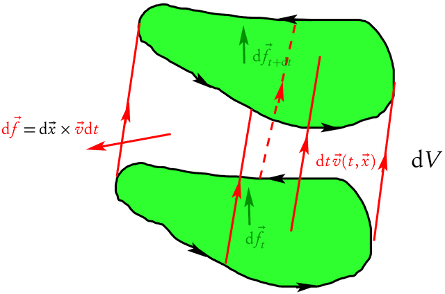
Now we use a trick to evaluate the second integral in (\ref{a.4}) further: We apply Gauss’s integral theorem to evaluate the integral of $\vec{\nabla} \cdot \vec{B}$ (forgetting for the moment that this expression vanishes due to Gauss’s Law for the magnetic field) over the infinitesimal volume depicted in the figure above. This volume is swept out by the surface $f$ during the infinitesimal time interval $(t,t+\dd t)$. It is like a cylinder of infinitesimal hight, i.e., it consists of the two surfaces $f(t+\dd t)$ (in Gauss’s integral theorem with the surface-element normal vector $\dd^2 \vec{f}_{t+\dd t}$) and $f(t)$ (surface-normal vector $-\dd^2 \vec{f}_{t}$ as well as on the infinitesimal mantle (with the surface-normal vector given by $\dd^2 \vec{f}=\dd t \dd \vec{x} \times \vec{v}$. The volume element itself can be written as $\dd t \dd^2 \vec{f} \cdot \vec{v}$. Thus, Gauss’s integral theorem gives to order $\mathcal{O}(\dd t^2)$
\begin{equation}
\begin{split}
\label{a.5}
\int_{\dd V} \dd^3 \vec{x} \vec{\nabla} \cdot \vec{B} &= \dd t
\int_{f(t)} \dd^2 \vec{f} \cdot \vec{v} (\vec{\nabla} \cdot \vec{B}) \\
&=
\int_{\partial V} \dd^2 \vec{f} \cdot \vec{B}=\int_{f(t+\dd t)} \dd^2
\vec{f} \cdot \vec{B} – \int_{f(t)} \dd^2 \vec{f} \cdot \vec{B} + \dd t
\int_{\partial f(t)} (\dd \vec{x} \times \vec{v}) \cdot \vec{B}.
\end{split}
\end{equation}
Thus we get
\begin{equation}
\label{a.6}
\int_{f(t+\dd t)} \dd^2
\vec{f} \cdot \vec{B} – \int_{f(t)} \dd^2 \vec{f} \cdot \vec{B} = \dd t
\int_{f(t)} \dd^2 \vec{f} \cdot \vec{v} (\vec{\nabla} \cdot \vec{B}) -\dd t
\int_{\partial f(t)} (\dd \vec{x} \times \vec{v}) \cdot \vec{B} +
\mathcal{O}(\dd t^2).
\end{equation}
Plugging this into (\ref{a.4}) and dividing by $\dd t$ leads to the
desired time derivative of the flux
\begin{equation}
\label{a.7}
\dot{\Phi}_{\vec{B}}=\int_{f(t)} \dd^2 \vec{f} \cdot [\partial_t \vec{B}
+ \vec{v} (\vec{\nabla} \cdot \vec{B})] – \int_{\partial f(t)} \dd
\vec{x} \cdot (\vec{v} \times \vec{B}).
\end{equation}
In the last integral we have used $(\dd \vec{x} \times \vec{v}) \cdot \vec{B}=\dd \vec{x} \cdot (\vec{v} \times \vec{B})$. Now using
$\vec{\nabla} \cdot \vec{B}=0$ and comparing with (\ref{a.2}) leads,
after some simple algebra, to the correct \textbf{Faraday Law of
Induction}, also known as the \textbf{flux law}:
\begin{equation}
\label{a.8}
\int_{\partial f(t)} \dd \vec{x} \cdot \left (\vec{E}+\frac{\vec{v}}{c}
\times \vec{B} \right )=-\frac{1}{c} \dot{\Phi}_{\vec{B}}(t).
\end{equation}

A pdf version of this article can be found at

https://th.physik.uni-frankfurt.de/~hees/pf-faq/homopolar.pdf