A Numerical Electromagnetic Solver Using Duality

In the previous insights article (How to Use Duality in Computational Electromagnetic Problems), I covered some uniqueness theorems for the Riemann-Silberstein vector, $F=E+iB$, for time-harmonic fields. We showed that the boundary value, $f$, completely determines the vector field throughout the volume. In this article, I’d like to step through constructing a numerical algorithm for finding $F$ given $f_\uparrow$.

I’ve never done a finite element program from scratch before. This seems as good a time as any to try one. The algorithm is based entirely on what we developed in the previous insights so it will look somewhat different than the usual ones. Hope you find this interesting.

Recap

Just so we have everything up front I’d like to remind everyone of the important bits we’ll be using. The linear vector space, $\Lambda_k(V),$ is the collection of all solutions to the differential equation, $$\nabla\times F + kF = 0,$$ on the volume, $V.$ The constant, $k=2\pi/\lambda$, is the wavenumber. It’s important to allow $k$ to be complex since this is how we model lossy materials. Conceivably there may also be applications where one model gains in materials and we wouldn’t want to leave these out either.

The convention we follow is to write fields on the volume using uppercase letters while the corresponding boundary values are written using the corresponding lower case letter. So for every $F\in\Lambda_k$ we have a unique boundary value, $f\in\lambda_k$. Our central result from the previous insights was $F=0 \iff f=0$.

The really magic thing we discovered along the way about these boundary values is they obey the integral relation, $$(f|N|g) = i(k^\ast_1-k_2)(F|G).$$ Here we’ve taken the general case where $f\in\lambda_{k_1}$ and $g\in\lambda_{k_2}.$ This is a general relation between the matrix elements of the hermitian operator, $N,$ on the surface, and the overlap integral on the volume of the corresponding fields. Okay, so? Well, notice if we take $k_1 = k^\ast$ and $k_2 = k$ we get the following truth, $$(f|N|g) = 0,$$ which holds for all values of $k$. What we have here are linear relations the elements $g\in\lambda_k$ must satisfy to be solution boundary values in the first place. Our numerical method will stem from insisting these relations hold for a modeling space of our choosing.

We need to unpack this last result a bit further. The operator $N$ is really central to this whole subject. Recall that it is just the boundary value obtained by crossing with the surface normal $\hat{n}$, $$N(g) = -i\hat{n}\times g.$$ $N$ has a number of interesting properties. For example we know $N^2=1$ so its eigenvalues are $\pm 1$. This led us to define the two orthogonal projectors, $P^\uparrow$ and $P^\downarrow.$ With these comes the unique split of any $f$ into orthogonal components, $$f = f^\uparrow + f^\downarrow.$$ Writing the matrix elements of $N$ out using this split gives, $$\boxed{(f^\uparrow|g^\uparrow) = (f^\downarrow|g^\downarrow)},$$ for all $k$ provided $f\in\lambda_{k^\ast}$ and $g\in\lambda_k$. We’ll be building our program using this relation so we’ve put it in a box where we can find it.

Representing $V$

First order of business we must choose a numerical representation for a general volume $V.$ Like so many things this choice is driven by practical consideration. People have spent lifetimes on just this problem so we’re going to use a publicly available software package called GMSH. This program generates tetrahedral meshes of some really complicated regions. There is a learning curve but it’s actually quite usable.

What’s a tetrahedral mesh? Well, a tetrahedron (called an element) is a convex four-sided figure specified by its 4 vertex points in space, $\{r_1,r_2,r_3,r_4\}.$ A tetrahedral mesh is a collection of tetrahedra that give us, $$V = \bigcup_n T_n.$$ Elements either don’t intersect or have one, two, or three vertices in common. We are only interested when two tetrahedra share 3 vertex points. This is where have a face in common.

Field Representation

In principle, we only really need to know or talk about the field boundary values on each element. It’s really useful to introduce basis sets that are confined to each face. Doing this makes it really easy to share an element’s boundary values with its neighbors. This also provides us a field representation as a finite set of numbers, something that’s essential if we’re going to be using computers.

We already have a natural split between $\uparrow$ and $\downarrow$-components. Given a face we must choose or decide on some number, $N_b$, of $\downarrow$-basis or fitting functions we’re going to include. Natural choices at this stage are $N_b=1$ recommended by its deceptive simplicity. I can make $N_b=1$ work, but it’s not as natural or as simple as it might first appear. I’m actually going to reject $N_b=1$ for the same reason I going to reject $N_b=4.$ The reason is the error incurred for an element by truncating to either of these dimensions ends up being anisotropic at some level. For $N_b=2$ or $3$ the errors incurred can be made isotropic. The choice $N_b=2$ is possible but not very convenient. This leaves me with one option, $N_b=3.$

Having looked at face basis for some time there is a particular basis set I have in mind. Defining them takes a step that appears kind of goofy at first. We want to embed each face in a complex plane. Simple to do by picking two orthogonal unit vectors in the plane of the face, say $\hat{x}$ and $\hat{y}.$ This will give each of the face vertices a complex number location, $$z_i = r_i\cdot(\hat{x}+i\hat{y}).$$ With these I’m going to define 3 complex vector valued interpolation functions, $$\alpha_1(z) = \frac{1}{\sqrt{2}}\frac{(z-z_2)(z-z_3)}{(z_1-z_2)(z_1-z_3)}(\hat{x}+i\hat{y}).$$ I’ve only written the first one out. The other two are gotten by cycling indices. Thing to keep in mind is these are really functions of location $\alpha_i(r)$ with $z=r\cdot(\hat{x}+i\hat{y}).$ If $r$ is on some other face then it is understood that $\alpha_i(r)=0$ by definition.

These basis elements have a number of noteworthy properties. The collection of $\alpha_i(r)$ for all of an elements faces gives us a truncated or approximate basis of $\lambda_k^\uparrow$ for the element. They act as a kind of spline fit since, $$\alpha_i(r_j) = \frac{1}{\sqrt{2}}(\hat{x}+i\hat{y})\delta_{ij}.$$ Given a field, $F,$ we write an approximation of its boundary value, $f^\uparrow,$ as, $$f^\uparrow(r) \simeq \sum_{n=1}^{12} a_n\alpha_n(r),$$ where the fitting coefficients are, $$a_n = F(r_n)\cdot \alpha_n(r_n)$$ We can do the same for $f^\downarrow$ by noting the corresponding basis for $\lambda_k^\downarrow$ is just $\beta_i = \alpha_i^\ast.$

This gives us the approximate representation for a field we’ll be using in our algorithm. A general field is specified by 6 complex coefficients per face. These numbers are not all independent. In fact, given just 3 of these coefficients per face on the boundary of the mesh will allow us to compute the remaining ones.

There are two other properties of these functions we should mention before moving on. The first is they are second-order polynomials in $z.$ Turns out any second-order polynomial that takes on the same value at three distinct points is identically a constant. Why this is important has to do with what is known as the patch test[1] in Finite Element Analysis. The basic upshot of the patch test is any basis (aka shape functions) that can’t approximate a constant is doomed to fail (or at best suck). The reasons for this are apparent. In the limit of very small elements, we need to be able to approximate nearly constant fields. If your basis doesn’t contain a constant then you’re out of luck.

The second property is that $\alpha$’s and $\beta$’s are really closely related to local solutions to our differential equation. If one multiplies an $\alpha$ by the phase factor $e^{-ik\hat{n}\cdot r}$ and extends into the element, then it obeys the field equation. This really justifies calling $\alpha_i$ out-ports and the $\beta_i$ in-ports because they refer to incoming and outgoing wavefronts.

[1] In FEM this a known as the patch test. If your selected basis set can’t model a constant, expect trouble. See “The Finite Element Method”, 3’rd edition, by Zienkiewicz 

The Element $S$-matrix

Our boxed relation makes it clear that the field expansion coefficients $a_n$ and $b_n$ are not independent for an element. Let’s consider the case where a single $b_n=1$ and the remaining $b$’s are 0. In this case we have, $$f_n \simeq \beta_n + \sum_{m=1}^{12}S_{nm}\alpha_m.$$ The matrix $S_{nm}$ are 144 complex numbers we need to determine for each element in our mesh. What we require are 12 known elements of $E_l\in\Lambda_{k^\ast}$ that are linearly independent. Plugging these into our boxed relation yields a matrix equation, $$AS = B,$$ where $A_{lm}=(e_l|\alpha_m)$ and $B_{ln} = (e_l|\beta_n).$ If $A$ is invertible then the solution is just,$$S=A^{-1}B.$$ Gee, this looks nice. Okay, will any linearly independent 12 vectors chosen at random from the infinite dimensional box $\Lambda_{k^\ast}$ do? In exact arithmetic possibly maybe? Fine, in real life then? Yeah, no definitely not.

Choosing Our Vectors

A really attractive notion is to choose $\langle E_l\rangle$ as a rotationally invariant vector space. The penalty for not doing so affects the $S$-matrix one obtains. If a rotation changes the space $\langle E_l\rangle$ then the $S$-matrix obtained will also change by some amount. Picking a rotationally invariant space insures this doesn’t happen. It also allows us to lift them wholesale from a book. For all my function needs I turn to the second edition of Brink and Satchler. From Equation 4.44 on page 68 it’s easy to see, $$F_{lm} = \nabla\times\mathbf{L}\phi_{lm} – k\mathbf{L}\phi_{lm},$$ are the functions we need.

Like all things angular momentum, $l=1,2,\cdots,$ while the magnetic quantum number, $m=l,l-1,\cdots, -l.$ For each $l$ we have $2l+1$ vectors all related by rotations. No single value of $l$ works for us, but two taken together still gives an invariant subspace. There are only 2 possibilities for $N_b=3$,  $l=1\text{ and }4$$$\langle E_n\rangle = \langle F_{1m}\rangle\oplus \langle F_{4m}\rangle$$ or $l=2\text{ and }3,$ $$\langle E_n\rangle = \langle F_{2m}\rangle\oplus \langle F_{3m}\rangle.$$

The Full S-Matrix

We now want to assemble these into one gigantic sparse matrix for our mesh. The place to start with this is with a single tetrahedron. Our discretized $F$ in this case is a 24 element column vector containing 12 a’s and 12 b’s. Writing the full $S$-matrix out in block form, $$ \left(\begin{array}{cc} 0 & 0 \\ S_{nm} & 0\end{array}\right)\left(\begin{array}{c}a_m\\b’_m\end{array}\right)=\left(\begin{array}{c}0\\b_n\end{array}\right).$$

Several things are going on here that need to be pointed out. First, the $b_m$ on the right are determined by applying the $S_{nm}$ block to the $a_m$ on the left. Second, the $b’_m$ on the left doesn’t affect the resulting vector on the right at all. Applying the matrix $S$ the $a_m$ are zeroed out.

With only one tetrahedron, every face is a boundary face. As we add more tetrahedrons, interior faces are added. Interior faces behave a little differently.

For a single tetrahedron  $F$ is determined by the equation, $$F=A_o+SF$$ where $A_o$ is a column vector containing just the boundary a’s. This equation remains valid as we add tetrahedra to the model. It’s easy to check for the single element mesh that $F=0$ if and only if $A_o=0$.

An essential step is to make a matrix plan. This plan is basically what will go into our data structure when we get around to implementing our algorithm which, by the way, we have yet to define.

We need to assign a unique index to each face. For each face, we need to have the index of the tetrahedron on the front of the face and the index of the tetrahedron on the back of the face. If one of the tetrahedrons is missing the index is taken as zero (yes, yes we’re using Fortran) and we have a boundary element. The final bit of information we need is an indexed list of tetrahedrons which contains the 4 face indices making up each tetrahedron.

The System Equation

Okay, we have a discretized $F$ which is a column vector indexed by a coefficient.

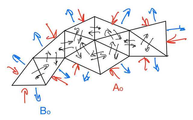
Figure 1 – Schematic of a tetrahedral mesh.

 

First off we need some diagrams. Figure (1) shows tetrahedrons schematically as triangles. The red arrows are the a’s and the blue arrows are the b’s. The full system S maps each tetrahedron a’s into its b’s. For interior faces (shown as black arrows) the $a$’s and $b$’s play both roles. The output of a tetrahedron is the input of its neighbors and vice versa. For boundary elements things are different. Nothing maps into a’s on the boundary. Applying S doesn’t change or provide these values. Let us collect all the boundary a’s into a single vector where all other entries are 0. Call this vector, $A_o$, which is our drive vector.

Suppose we have a solution, $F$. The system equation for $F$ is, $$F = A_o + S F.$$ This equation is saying that applying $S$ to a solution gives us the solution back but peels off the drive vector, $A_o,$ in the process. To get the full $F$ back, we just add the missing bit back in.

Okay, How do we solve this?

Given a drive vector, how do we compute $F$? Well, there is the right way which is to factor and solve the sparse matrix equation, $$(\mathbf{1} – S)F = A_o,$$

which is somewhat tedious. There are excellent software libraries for this. My first inclination is to try an iterative solution like conjugate gradients or one of its variants. We’ll see.

That’s it for now.

Well, this article is about as long as I can tolerate. At any rate, we’ve defined an algorithm that is complete enough to be coded and tested. The next installment of this series will hopefully include the code and results from testing. The plan is to provide the program and test cases on Github.

Comment Thread