Examples of Prequantum Field Theories I: Gauge Fields

 

 

After having motivated the need for prequantum field theory and having laid out its principles (i. extremal action, ii. global action, iii. covariant phase space, iv. local observables), it is time to look at examples. The key classes of examples — which are considerably larger than one may think — are 1) field theories of Chern-Simons type and 2) field theories of Wess-Zumino-Witten type. Before I discuss the construction of their prequantum Lagrangians, we need to have a close look at their field bundles. In general, these are higher smooth stacks of higher gauge fields. Before I get to that, in turn, it serves to have a fresh look at the familiar gauge fields. This is what we do now.

---

 

Modern physics rests on two fundamental principles. One is the locality principle; its mathematical incarnation in terms of differential cocycles on PDEs was the content of the previous articles. The other is the gauge principle.

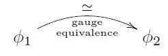
In generality, the gauge principle says that given any two field configurations $\phi_1$ and $\phi_2$, then it is physically meaningless to ask whether they are equal, instead one has to ask whether they are equivalent via a gauge transformation.

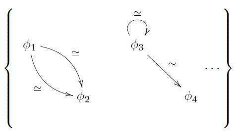
There may be more than one gauge transformation between two field configurations, and hence there may be auto-gauge equivalences that non-trivially re-identify a field configuration with itself.  Hence a space of physical field configurations does not really look like a set of points, it looks more like this cartoon:

 

Moreover, if there are two gauge transformations, it is again physically meaningless to ask whether they are equal, instead one has to ask whether they are equivalent via a gauge-of-gauge transformation.

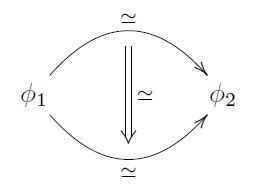
And so on.

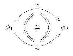
In this generality, the gauge principle of physics is the mathematical principle of homotopy theory: in general it is meaningless to say that some objects form a set, instead one has to consider the groupoid which they form, whose morphisms are the equivalences between these objects. Moreover, in general, it is wrong to assume that any two such morphisms are equal or not, rather one has to consider the groupoid which these form, which then in total makes a 2-groupoid. But in general, it is also meaningless to ask whether two equivalences of two equivalences are equal or not, and continuing this way one finds that objects in the general form an infinity-groupoid, also called a homotopy type.

For more background on this, see the lecture notes at the geometry of physics — homotopy types.

Of particular interest in physics are smooth gauge transformations that arise by the integration of infinitesimal gauge transformations. An infinitesimal smooth groupoid is a Lie algebroid and an infinitesimal smooth $\infty$-groupoid is an infinity-Lie algebroid. The importance of infinitesimal symmetry transformations in physics, together with the simple fact that they are easier to handle than finite transformations, makes them appear more prominently in the physics literature. In particular, the physics literature is secretly well familiar with smooth $\infty$-groupoids in their infinitesimal incarnation as $\infty$-Lie algebroids: these are equivalently what in physics is called BRST complexes. What are called ghosts in the BRST complex are the cotangents to the space of equivalences between objects, and what are called higher-order ghosts-of-ghosts are cotangents to spaces of higher-order equivalences-of-equivalences. We indicate in a moment how to see this.

 

While every species of fields in physics is subject to the gauge principle, one speaks specifically of gauge fields for those fields which are locally given by differential forms $A$ with values in a Lie algebra (for ordinary gauge fields) or more generally with values in an $L_\infty$-algebroid (for higher gauge fields).  We now survey how such gauge fields come about.

 

---

 

 

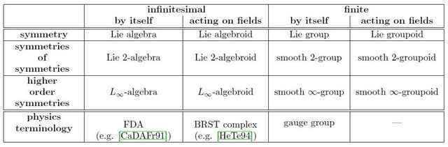
To start with, consider a plain group $G$. For the standard applications mentioned in The need for Prequantum geometry we would take $G = U(1)$ or $G = \mathrm{SU}(n)$ or products of these.

In order to highlight that we think of $G$ as a group of symmetries acting on some (presently unspecified object) $\ast$, we write

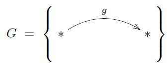
In this vein, the product operation $(-)\cdot (-) : G \times G \to G$ in the group reflects the result of applying two symmetry operations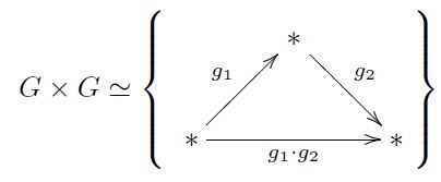

Similarly, the associativity of the group product operation reflects the result of applying three symmetry operations:

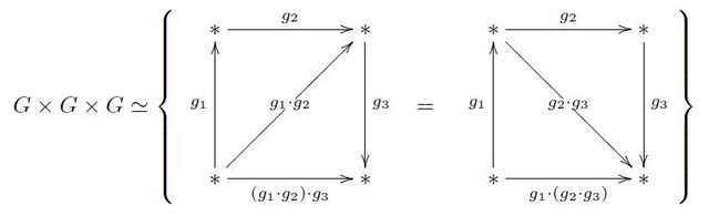
Here the reader should think of the diagram on the right as a tetrahedron, hence a 3-simplex, that has been cut open only for notational purposes.

Continuing in this way, $k$-tuples of symmetry transformations serve to label $k$-simplices whose edges and faces reflect all the possible ways of consecutively applying the corresonding symmetry operations. This forms a simplicial set, called the simplicial nerve of $G$, hence a system
$$
\mathbf{B}G
:
k \mapsto G^{\times_k}
$$
of sets of $k$-simplices for all $k$, together with compatible maps between these that restrict $k+1$-simplices to their $k$-faces (the face maps) and those that regard $k$-simplices as degenerate $k+1$-simplices (the degeneracy maps). From the above picture, the face maps of $\mathbf{B}G$ in low degree look as follows (where $p_i$ denotes projection onto the $i$th factor in a Cartesian product):

It is useful to remember the smooth structure on these spaces of $k$-fold symmetry operation by remembering all possible ways of forming smoothly $U$-parameterized collections of $k$-fold symmetry operations, for any abstract coordinate chart $U = \mathbb{R}^n$. Now a smoothly $U$-parameterized collection of $k$-fold $G$-symmetries is simply a smooth function from $U$ to $G^{\times_k}$, hence equivalently is $k$ smooth functions from $U$ to $G$. Hence the symmetry group $G$ together with its smooth structure is encoded in the system of assignments
$$
\mathbf{B}G : (U,k) \mapsto C^\infty(U, G^{\times_k}) = C^\infty(U,G)^{\times_k}
$$
which is contravariantly functorial in abstract coordinate charts $U$ (with smooth functions between them) and in abstract $k$-simplices (with cellular maps between them). This is the incarnation of $\mathbf{B}G$ as a smooth simplicial presheaf.

For more on how these work see the lecture notes geometry of physics — smooth homotopy types.

Another basic example of a smooth simplicial presheaf is the nerve of an open cover. Let $\Sigma$ be a smooth manifold and let $\{U_i \longrightarrow \Sigma\}_{i \in I}$ be a cover of $\Sigma$ by coordinate charts $U_i \simeq \mathbb{R}^n$. Write $U_{i_0 \cdots i_k} := U_{i_0} \underset{X}{\times} U_{i_1} \underset{X}{\times} \cdots \underset{X}{\times} U_{i_k}$ for the intersection of $(k+1)$ coordinate charts in $X$. These arrange into a simplicial object like so:

A map of simplicial objects
$$
C(U_i) \longrightarrow \mathbf{B}G
$$
is in degree 1 a collection of smooth $G$-valued functions $g_{i j} : U_{i j} \longrightarrow G$ and in degree 2 it is the condition that on $U_{i j k}$ these functions satisfy the cocycle condition $g_{i j} g_{j k} = g_{i k}$. Hence this defines the transition functions for a $G$-principal bundle on $\Sigma$. In physics this may be called the instanton sector of a $G$-gauge field. A $G$-gauge field itself is a connection on such a $G$-principal bundle, we come to this in a moment.

We may also think of the manifold $\Sigma$ itself as a simplicial object, one that does not actually depend on the simplicial degree. Then there is a canonical projection map $C(\{U_i\}) \stackrel{\simeq}{\longrightarrow} \Sigma$. When restricted to arbitrarily small open neighbourhoods (stalks) of points in $\Sigma$, then this projection becomes a weak homotopy equivalence of simplicial sets. We are to regard smooth simplicial presheaves which are connected by morphisms that are stalkwise weak homotopy equivalences as equivalent. With this understood, a smooth simplicial presheaf is also called a higher smooth stack or a smooth infinity-groupoid. Hence a $G$-principal bundle on $\Sigma$ is equivalently a morphism of higher smooth stacks of the form
$$
\Sigma \longrightarrow \mathbf{B}G
\,.
$$

For more on this see the lecture notes geometry of physics — principal bundles.

 

---

 

For analysing smooth symmetries it is useful to focus on infinitesimal symmetries. To that end, consider the (first-order) infinitesimal neighbourhood $\mathbb{D}_e(-)$ of the neutral element in the simplicial nerve. Here $\mathbb{D}_e(-)$ is the space around the neutral element that is “so small” that for any smooth function on it which vanishes at $e$, the square of that function is “so very small” as to actually be equal to zero.

For more on infinitesimal geometry see super Cartan geometry — the geometric substance. For a textbook that presents all of the traditional differential geometry from this point of view see [Kock 10].

We denote the resulting system of $k$-fold infinitesimal $G$-symmetries by $\mathbf{B}\mathfrak{g}$:

The alternating sum of pullbacks along the simplicial face maps shown above defines a differential $d_{\mathrm{CE}}$ on the spaces of functions on these infinitesimal neighbourhoods. The corresponding normalized chain complex is the differential-graded algebra on those functions which vanish when at least one of their arguments is the neutral element in $G$. One finds that this is the Chevalley-Eilenberg algebra
$$
\mathrm{CE}(\mathbf{B}\mathfrak{g})
=
\left(
\wedge^\bullet \mathfrak{g}^\ast,
\;
d_{\mathrm{CE}} = [-,-]^\ast
\right)
\,,
$$
which is the Grassmann algebra on the linear dual of the Lie algebra $\mathfrak{g}$ of $G$ equipped with the differential whose component $\wedge^1 \mathfrak{g}^\ast \to \wedge^2 \mathfrak{g}^\ast$ is given by the linear dual of the Lie bracket $[-,-]$, and which hence extends to all higher degrees by the graded Leibnitz rule.

For example, when we choose $\{t_a\}$ a linear basis for $\mathfrak{g}$, with structure constants of the Lie bracket denoted $[t_a,t_b] = C^c{}_{a b} t_c$, then with a dual basis $\{t^a\}$ of $\mathfrak{g}^\ast$ we have that
$$
d_{\mathrm{CE}} t^a = \tfrac{1}{2} C^a{}_{b c} \, t^b \wedge t^c
\,.
$$
Given any structure constants for a skew bracket like this, then the condition $(d_{\mathrm{CE}})^2 = 0$ is equivalent to the Jacobi identity, hence to the condition that the skew bracket indeed makes a Lie algebra.

Traditionally, the Chevalley-Eilenberg complex is introduced in order to define and to compute Lie algebra cohomology: a $d_{\mathrm{CE}}$-closed element
$$
\mu \in \wedge^{p+1} \mathfrak{g}^\ast \hookrightarrow \mathrm{CE}(\mathfrak{g})
$$
is equivalently a Lie algebra $(p+1)$-cocycle. This phenomenon will be crucial further below.

Thinking of $\mathrm{CE}(\mathbf{B}\mathfrak{g})$ as the algebra of functions on the infinitesimal neighbourhood of the neutral element inside $\mathbf{B}G$ makes it plausible that this is an equivalent incarnation of the Lie algebra of $G$. This is also easily checked directly: sending finite-dimensional Lie algebras to their Chevalley-Eilenberg algebra constitutes a fully faithful inclusion
$$
\mathrm{CE}
\;:\;
\mathrm{LieAlg}
\hookrightarrow
\mathrm{dgcAlg}^{\mathrm{op}}
$$
of the category of Lie algebras into the opposite of the category of differential graded-commutative algebras. This perspective turns out to be useful for computations in gauge theory and in higher gauge theory. Therefore it serves to see how various familiar constructions on Lie algebras look when viewed in terms of their Chevalley-Eilenberg algebras.

Most importantly, for $\Sigma$ a smooth manifold and $\Omega^\bullet(\Sigma)$ denoting its de Rham dg-algebra of differential forms, then flat $\mathfrak{g}$-valued 1-forms on $\Sigma$ are equivalent to dg-algebra homomorphisms like so:
$$
\Omega^\bullet_{\mathrm{flat}}(\Sigma,\mathfrak{g})
:=
\left\{
A \in \Omega^1(\Sigma)\otimes \mathfrak{g} \;|\; F_A := d_{\mathrm{dR}}A – \tfrac{1}{2}[A \wedge A] = 0
\right\}
\;\simeq\;
\left\{
\;\;
\Omega^\bullet(\Sigma)
\longleftarrow
\mathrm{CE}(\mathbf{B}\mathfrak{g})
\;\;
\right\}
\,.
$$
To see this, notice that the underlying homomorphism of graded algebras $\Omega^\bullet(\Sigma) \longleftarrow \wedge^\bullet \mathfrak{g}^\ast$ is equivalently a $\mathfrak{g}$-valued 1-form, and that the respect for the differential forces it to be flat:

 

---

 

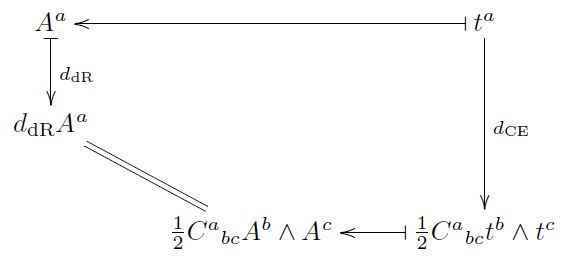
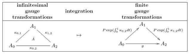
The flat Lie algebra valued forms play a crucial role in recovering a Lie group from its Lie algebra as the group of finite paths of infinitesimal symmetries. To that end, write $\Delta^1 := [0,1]$ for the abstract interval. Then a $\mathfrak{g}$-valued differential form $A \in \Omega^1_{\mathrm{flat}}(\Delta^1,\mathfrak{g})$ is at each point of $\Delta^1$ an infinitesimal symmetry, hence it encodes the finite symmetry transformation that is given by applying the infinitesimal transformation $A_t$ at each $t \in \Delta^1$ and then “integrating these”. This integration is called the parallel transport of $A$ and is traditionally denoted by the symbols $P \exp(\int_0^1 A) \in G$. Now of course different paths of infinitesimal transformations may have the same integrated effect. But precisely if $A_1$ and $A_2$ have the same integrated effect, then there is a flat $\mathfrak{g}$-valued 1-form on the disk which restricts to $A_1$ on the upper semicircle and to $A_2$ on the lower semicircle.

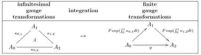
In particular, the composition of two paths of infinitesimal gauge transformations is in general not equal to any given such path with the same integrated effect, but there will always be a flat 1-form $\hat A$ on the 2-simplex $\Delta^2$ which interpolates

 

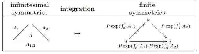
In order to remember how the group obtained this way is a Lie group, we simply need to remember how the above composition works in smoothly $U$-parameterized collections of 1-forms. But a $U$-parameterized collection of 1-forms on $\Delta^k$ is simply a 1-form on $U \times \Delta^k$ which vanishes on vectors tangent to $U$, hence a vertical 1-form on $U \times \Delta^k$, regarded as a simplex bundle over $U$.

All this is captured by saying that there is a smooth simplicial presheaf $\exp(\mathfrak{g})$ which assigns to an abstract coordinate chart $U$ and a simplicial degree $k$ the set of flat vertical $\mathfrak{g}$-valued 1-forms on $U \times \Delta^k$:
$$
\begin{aligned}
\exp(\mathfrak{g}) :=
(U,k)
\;\;
& \mapsto
\Omega^\bullet_{\mathrm{flat} \atop \mathrm{vert}}( U \times \Delta^k,\mathfrak{g})
\\
& =
\left\{
\;
\Omega^\bullet_{\mathrm{vert}}(U \times \Delta^k)
\longleftarrow
\mathrm{CE}(\mathbf{B}\mathfrak{g})
\;
\right\}
\end{aligned}
\,.
$$
By the above discussion, we do not care which of various possible flat 1-forms $\hat A$ on 2-simplices are used to exhibit the composition of finite gauge transformation. The technical term for retaining just the information that there is any such 1-form
on a 2-simpled at all is to form the 3-coskeleton $\mathrm{cosk}_3(\exp(\mathfrak{g}))$. And one finds that this indeed recovers the smooth gauge group $G$, in that there is a weak equivalence of simplicial presheaves:
$$
\mathrm{cosk}_3(\exp(\mathfrak{g}))
\simeq
\mathbf{B}G
\,.
$$

For more on this see the nLab at Lie integration.

 

---

 

 

So far this produces the gauge group itself from the infinitesimal symmetries. We now discuss how similarly its action on gauge fields is obtained. To that end, consider the Weil algebra of $\mathfrak{g}$, which is obtained from the Chevalley-Eilenberg algebra by throwing in another copy of $\mathfrak{g}$, shifted up in degree
$$
W(\mathfrak{g})
:=
\left(
\wedge^\bullet( \mathfrak{g}^\ast \oplus \mathfrak{g}^\ast[1] ), d_W = d_{\mathrm{CE}} + \mathbf{d}
\right)
\,,
$$
where $\mathbf{d} : \wedge^1 \mathfrak{g}^\ast \stackrel{\simeq}{\to} \mathfrak{g}^\ast[1]$ is the degree shift and we declare $d_{\mathrm{CE}}$ and $\mathbf{d}$ to anticommute. So if $\{t^a\}$ is the dual basis of $\mathfrak{g}^\ast$ from before, write $\{r^a\}$ for the same elements thought of in one degree higher as a basis of $\mathfrak{g}^\ast[1]$; then
$$
\begin{aligned}
d_{\mathrm{W}} & : t^a \;\mapsto\; \tfrac{1}{2}C^a{}_{b c} t^b \wedge t^c + r^a
\\
d_{\mathrm{W}} & : r^a \;\mapsto\; C^a{}_{b c} t^b \wedge r^c
\end{aligned}
\,.
$$
A key point of this construction is that dg-algebra homomorphisms out of the Weil algebra into a de Rham algebra are equivalent to unconstrained $\mathfrak{g}$-valued differential forms:
$$
\Omega(\Sigma,\mathfrak{g})
:=
\left\{
A \in \Omega^1(\Sigma)\otimes \mathfrak{g}
\right\}
\;\;\simeq\;\;
\left\{
\;\;
\Omega^\bullet(\Sigma)
\longleftarrow
\mathrm{W}(\mathbf{B}\mathfrak{g})
\;\;
\right\}
\,.
$$
This is because now the extra generators $r^a$ pick up the failure of the respect for the $d_{\mathrm{CE}}$-differential, that failure is precisely the curvature $F_A$:

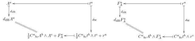
Notice here that once $t^a \mapsto A^a$ is chosen, then the diagram on the left uniquely specifies that $r^a \mapsto F_A^a$ and then the diagram on the right is already implied: its commutativity is the Bianchi identity $d F_A = [A\wedge F_A]$ that is satisfied by curvature forms.

Traditionally, the Weil algebra is introduced in order to define and compute invariant polynomials on a Lie algebra.
A $d_{\mathrm{W}}$-closed element in the shifted generators
$$
\langle -,-,\cdots\rangle \in \wedge^{k} \mathfrak{g}^\ast[1] \hookrightarrow \mathrm{W}(\mathbf{B}\mathfrak{g})
$$
is equivalently an invariant polynomial of order $k$ on the Lie algebra $\mathfrak{g}$. Therefore write $\mathrm{inv}(\mathfrak{g})$ for the graded commutative algebra of invariant polynomials,  thought of as a dg-algebra with vanishing differential.

For convenience, for the remainder of this article we abuse notation and write $\mathrm{CE}(\mathfrak{g})$ and $\mathrm{W}(\mathfrak{g})$ instead of $\mathrm{CE}(\mathbf{B}\mathfrak{g})$ and $W(\mathbf{B}\mathfrak{g})$, respectively.

There is a canonical projection map from the Weil algebra to the Chevalley-Eilenberg algebra,  given simply by forgetting the shifted generators ($t^a \mapsto t^a$; $r^a \mapsto 0$). And there is the defining inclusion  $\mathrm{inv}(\mathfrak{g}) \hookrightarrow \mathrm{W}(\mathfrak{g})$.

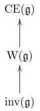
Cartan had introduced all these dg-algebras as algebraic models of the universal $G$-principal bundle. We had seen above that homomorphisms $\Omega^\bullet_{\mathrm{vert}}(U \times \Delta^k) \longleftarrow \mathrm{CE}(\mathfrak{g})$ constitute the gauge symmetry group $G$ as integration of the paths of infinitesimal symmetries. Here the vertical forms on $U \times \Delta^k$ are themselves part of the sequence of differential forms on the trivial $k$-simplex bundle over the given coordinate chart $U$. Hence consider compatible dg-algebra homomorphisms between these two sequences:

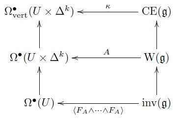
We unwind what this means in components: The middle morphism is an unconstrained Lie algebra valued form $A\in \Omega^1(U \times \Delta^k, \mathfrak{g})$, hence is a sum
$$
A = A_U + A_{\Delta^k}
$$
of a 1-form $A_U$ along $U$ and 1-form $A_{\Delta^k}$ along $\Delta^k$.  The second summand $A_{\Delta^k}$ is the vertical component of $A$. The commutativity of the top square above says that as a vertical differential form, $A_{\Delta^k}$ has to be flat. By the previous discussion this means that $A_{\Delta^k}$ encodes a $k$-tuple of $G$-gauge transformations. Now we will see how these gauge transformations naturally act on the  gauge field $A_U$:

Consider this for the case $k = 1$, and write $t$ for the canonical coordinate along $\Delta^1 = [0,1]$.  Then $A_U$ is a smooth $t$-parameterized collection of 1-forms, hence of $\mathfrak{g}$-gauge fields, on $U$; and $A_{\Delta^1} = \kappa \,d t$ for $\kappa$ a smooth Lie algebra valued function, called the gauge parameter. Now the equation for the $t$-component of the total curvature $F_A$ of $A$ says how the gauge parameter together with the mixed curvature component causes infinitesimal transformations of the gauge field $A_U$ as $t$ proceeds:
$$
\frac{d}{dt} A_U = d_U \kappa – [\kappa, A] + \iota_{\partial_t} F_A
\,.
$$
But now the commutativity of the lower square above demands that the curvature forms evaluated in invariant polynomials have vanishing contraction with $\iota_t$. In the case that $\mathfrak{g} = \mathbb{R}$ this means that $\iota_{\partial t} F_A = 0$, while for nonabelian $\mathfrak{g}$ this is still generically the necessary condition. So for vanishing $t$-component of the curvature the above equation says that
$$
\frac{d}{dt} A_U = d\kappa – [\kappa, A]
\,.
$$
This is the traditional formula for infinitesimal gauge transformations $\kappa$ acting on  a gauge field $A_U$. Integrating this up, $\kappa$ integrates to a gauge group element $g := P \exp(\int_0^1 \kappa d t)$ by the previous discussion, and this equation becomes the formula for finite gauge transformations (where we abbreviate now $A_t := A_U(t)$):
$$
A_1
=
g^{-1} A_0 g + g^{-1} d_{\mathrm{dR}}g
\,.
$$
This gives the smooth groupoid $\mathbf{B}G_{\mathrm{conn}}$ of $\mathfrak{g}$-gauge fields with $G$-gauge transformations between them:

This dg-algebraic picture of gauge fields with gauge transformations between them now immediately generalizes to higher gauge fields with higher gauge transformations between them. Moreover, this picture allows producing prequantized higher Chern-Simons-type Lagrangians by Lie integration of transgressive $L_\infty$-cocycles. This I discuss in the next articles.

For more on the above see also the first pages of [Sati-Schreiber-Stasheff 09] and [Fiorenza-Schreiber-Stasheff 10].

Click For Forum Comments