Higher Prequantum Geometry IV: The Covariant Phase Space – Transgressively

The Euler-Lagrange ##p##-gerbes discussed in the previous article are singled out as being exactly the right coherent refinement of locally defined local Lagrangians that may be integrated over a ##(p+1)##-dimensional spacetime/worldvolume to produce a function, the action functional. In a corresponding manner, there are further refinements of locally defined Lagrangians by differential cocycles that are adapted to integration over submanifolds of ##\Sigma_{p+1}## of positive codimension. In codimension ##k## these will yield not functions, but ##p-k##-gerbes.

We consider this now for codimension 1 and find the covariant phase space of a locally variational field theory
equipped with its canonical (pre-)symplectic structure and equipped with a Kostant-Souriau prequantization of that.

As throughout, the following is indebted to discussion with Igor Khavkine.

First, consider the process of transgression in general codimension. In the convenient language of sheaves on smooth manifolds, it has the following simple incarnation.

Given a smooth manifold ##\Sigma##, then the mapping space ##[\Sigma,\mathbf{\Omega}^{p+1}]## into the smooth moduli space of ##(p+1)##-forms  is the smooth space defined by the property that for any other smooth manifold ##U##, there is a natural identification
$$
\left\{
U \longrightarrow [\Sigma, \mathbf{\Omega}^{p+1}]
\right\}
\;\;
\simeq
\;\;
\Omega^{p+1}(U \times \Sigma)
$$
of smooth maps into the mapping space with smooth ##(p+1)##-forms on the product manifold ##U \times \Sigma##.

Now suppose that ##\Sigma = \Sigma_{p+1-k}## is a compact oriented smooth manifold of dimension ##p+1-k##. Then there is the fiber integration of differential forms on ##U \times \Sigma## over ##\Sigma## (e.g. [Bott-Tu]), which gives a map
$$
\int_{(U \times \Sigma_{p+1-k}) / U} : \Omega^{p+1}(U \times \Sigma_{p+1-k}) \longrightarrow \Omega^{k}(U)
\,.
$$
This map is natural in ##U##, meaning that it is compatible with the pullback of differential forms along with any smooth functions ##U_1 \to U_2##. This property is precisely what is summarized by saying that the fiber integration map constitutes a morphism in the sheaf topos
$$
\int_\Sigma : [\Sigma_{p+1-k}, \mathbf{\Omega}^{p+1}] \longrightarrow \mathbf{\Omega}^{k}
$$
This provides an elegant means to speak about transgression. Namely given a differential form ##\alpha \in \Omega^{p+1}(X)## (on any smooth space ##X##) modulated by a morphism ##\alpha : X \longrightarrow \mathbf{\Omega}##, then its transgression to the mapping space ##[\Sigma,X]## is simply the form in ##\Omega^{p+1-k}([\Sigma,X])## which is modulated by the composite
$$
\int_{\Sigma} [\Sigma, -]
\;:\;
[\Sigma,X]
\stackrel{[\Sigma,\alpha]}{\longrightarrow}
[\Sigma, \mathbf{\Omega}^{p+1}]
\stackrel{\int_{\Sigma}}{\longrightarrow}
\mathbf{\Omega}^{k}
$$
of the fiber integration map above with the image of ##\alpha## under the functor ##[\Sigma,-]## that forms mapping spaces out of ##\Sigma##.

All this works verbatim also in the context of PDEs over ##\Sigma##. For instance if ##L : E \longrightarrow \mathbf{\Omega}^{p+1}_H## is a local Lagrangian on (the jet bundle of) a field bundle ##E## over ##\Sigma_{p+1}## as before, then the action functional that it induces, as in the previous article, is the transgression to ##\Sigma_{p+1}##:
$$
S : [\Sigma,E]_\Sigma \stackrel{[\Sigma,L]_\Sigma}{\longrightarrow} [\Sigma, \mathbf{\Omega}^{p+1}_H]_\Sigma
\stackrel{\int_\Sigma}{\longrightarrow} \mathbf{\Omega}^0
\,.
$$
But now the point is that we have the analogous construction in higher codimension ##k##, where the Lagrangian does not
integrate to a function (a differential 0-form) but to a differential ##k##-form.

And all this goes along with passing from globally defined differential forms to Cech-Deligne cocycles.

For more background and more details see also the lecture notes at

• geometry of physics — differential forms
• geometry of physics — integration

To apply this for codimension ##k = 1##, consider now ##p##-dimensional submanifolds ##\Sigma_p \rightarrow \Sigma## of spacetime/worldvolume. Write ##N^\infty_\Sigma \Sigma_p## for the formal normal neighbourhood of ##\Sigma_p## in ##\Sigma##, i..e. the infinitesimal thickening of ##Sigma_p## inside ##\Sigma##. In practice one is often, but not necessarily, interested in ##\Sigma_p## being a Cauchy surface, which means that the induced restriction map

$$
[\Sigma_{p+1},\mathcal{E}]
\longrightarrow
[N^\infty_\Sigma \Sigma_p, \mathcal{E}]
$$
(from field configurations solving the equations of motion on all of ##\Sigma## to normal jets of solutions on ##\Sigma_p##) is an equivalence. An element in the solution space ##[\Sigma_{p+1},\mathcal{E}]## is a classical state of the physical system that is being described, a classical trajectory of a field configuration over all of spacetime. Its image in ##[N^\infty_\Sigma\Sigma_{p},\mathcal{E}]## is the restriction of that field configuration and of all its derivatives to ##\Sigma_p##.

In many — but not in all — examples of interest, classical trajectories are fixed once their first-order derivatives over a Cauchy surface are known. In these cases, the phase space may be identified with the cotangent bundle of the space of field configurations on the Cauchy surface
$$
[N^\infty_\Sigma \Sigma_p, \mathcal{E}]
\simeq
T^\ast [\Sigma_p, E]
\,.
$$
The expression on the right is often regarded as the definition of phase spaces.  But since the equivalence with the left-hand side does not hold generally, we will not restrict attention to this simplified case and instead consider the solution space ##[\Sigma,\mathcal{E}]_\Sigma## as the phase space. To emphasize this more general point of view, one sometimes speaks of the
covariant phase space. Here “covariance” refers to invariance under the action of the diffeomorphism group of ##\Sigma##, meaning here that no space/time split in the form of a choice of Cauchy surface is made (or necessary) to define the phase space, even if a choice of Cauchy surface is possible and potentially useful for parameterizing phase space in terms of initial value data.

Since the notation ##[N^\infty_\Sigma \Sigma_p, \mathcal{E}]_\Sigma## is getting a bit heavy, from now on we will notationally suppress the denotation of the infinitesimal normals and just write

$$[\Sigma_p, \mathcal{E}]_\Sigma := [N^\infty_\Sigma \Sigma_p, \mathcal{E}]\,.$$

Since the only sensible interpretation of the left hand is the right hand, no confusion should arise.

It is crucial that the covariant phase space ##[\Sigma,\mathcal{E}]_\Sigma## comes equipped with further geometric structure which remembers that this is not just any old space, but the space of solutions of a locally variational differential equation. To see how this comes about, let us write ##(\mathbf{\Omega}^{p+1}_{\mathrm{cl}})_{\Sigma}## for the  moduli space of all closed ##p+1##-forms on PDEs. This is to mean that if ##E## is a bundle over ##\Sigma##, and regarded as representing the space of solutions of the trivial PDE on sections of ##E##, then morphisms ##E \longrightarrow (\mathbf{\Omega}^{p+1})_{\Sigma}## are equivalent to closed differential ##(p+2)##-forms on the jet bundle of ##E##.
$$
\left\{
E \longrightarrow (\mathbf{\Omega}^{p+1})_\Sigma
\right\}
\;\;\simeq\;\;
\Omega^{p+1}_{\mathrm{cl}}(J^\infty_\Sigma E)
\,.
$$
The key now is that there is a natural filtration on these differential forms adapted to spacetime codimension.  This is part of a bigrading structure on differential forms on jet bundles known as the variational bicomplex . In its low stages it looks as follows:

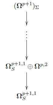
The lowest item here is what had concerned us in a previous article, it is the moduli of ##p+2##-forms which have ##p+1## of their legs along spacetime/worldvolume ##\Sigma## and whose remaining vertical leg along the space of local field configurations depends only on the field value itself, not on any of its derivatives. This was precisely the correct recipient of the variational curvature, hence the variational differential of horizontal ##(p+1)##-forms representing local Lagrangians.

But now that we are moving up in codimension, this coefficient will disappear, as these forms do not contribute when integrating just over ##p##-dimensional hypersurfaces. The correct coefficient for that case is instead clearly ##\mathbf{\Omega}^{p,2}##, the moduli space of those ##(p+2)##-forms on jet bundles which have ##p## of their legs along spacetime/worldvolume, and the remaining two along with the space of local field configurations.  (There is a more abstract way to derive this filtration from first principles,
and which explains why we have restriction to “source forms” (not differentially depending on the jets),
indicated by the subscript, only in the bottom row. But for the moment we just take that little subtlety for granted.)
So ##\mathbf{\Omega}^{p,2}## is precisely the space of those ##(p+2)##-forms on the jet bundle that become (pre-)symplectic 2-forms on the space of field configurations once evaluated on a ##p##-dimensional spatial slice ##\Sigma_p## of spacetime ##\Sigma_{p+1}##. We may think of this as a current on spacetime with values in 2-forms on fields.

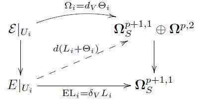
Indeed, there is a canonical such presymplectic current for every locally variational field theory [Zuckerman 87, Khavkine 14]. To see this, we ask for a lift of the purely horizontal locally defined Lagrangian ##L_i## through the variational bicomplex to a ##(p+1)##-form on the jet bundle whose curvature ##d(L_i + \Theta_i)## coincides with the Euler-Lagrange form ##\mathrm{EL} = \delta_V L_i## in vertical degree 1. Such a lift ##L_i + \Theta_i## is known as a Lepage form for ##L_i## (e.g. [GMS 09, 2.1.2]).

Notice that it is precisely the restriction to the shell ##\mathcal{E}## that makes the Euler-Lagrange form ##\mathrm{EL}_i## disappear, by construction, so that only the new curvature component ##\Omega_i## remains as the curvature of the Lepage form on the shell:

The condition means that the horizontal differential of ##\Theta_i## has to cancel against the horizontally exact part that appears when decomposing the differential of ##L_i## as discussed in a previous article. Hence, up to horizontal derivatives, this ##\Theta_i## is in fact uniquely fixed by ##L_i##:

$$
\begin{aligned}
d (L_i + \Theta_i) & = (\mathrm{EL}_i – d_H (\Theta_i + d_H(\cdots))) + (d_H \Theta_i + d_V \Theta_i)
\\
& = \mathrm{EL}_i + d_V \Theta_i
\\
& =: \mathrm{EL}_i + \Omega_i
\end{aligned}
\,.
$$
The new curvature component
$$
\Omega \in \Omega^{p,2}(J^\infty_\Sigma E)
$$
whose restriction to patches is given this way
$$
\Omega|_{U_i} := d_V \Theta_i
$$
is known as the presymplectic current [Zuckerman 87, Khavkine 14]. Because, by the way we  found its existence, this is such that its transgression over a codimension-1 submanifold ##\Sigma_p \longrightarrow \Sigma## yields a closed 2-form (a “presymplectic 2-form”) on the covariant phase space:
$$
\omega := \int_{\Sigma_p} [\Sigma_p, \Omega]
\in
\Omega^2([\Sigma_p, \mathcal{E}])
\,.
$$
Since ##\Omega## is uniquely specified by the local Lagrangians ##L_i##, this gives the covariant phase space canonically the structure of a presymplectic space ##([\Sigma,\mathcal{E}], \omega)##, and this is just the structure on phase space that reflects the fact that the phase space arises as the solutions to a locally variational classical field theory. This is the reason why phase spaces in classical mechanics are given by (pre-)symplectic geometry as in [Arnold 89].

But by the discussion in the previous article, we do not just consider a locally variational field classical field theory to start with, but a prequantum field theory. Hence in fact there is more data before transgression than just the new curvature components ##d_V \Theta_i##, there is also Cech cocycle coherence data that glues the locally defined ##\Theta_i## to a globally consistent differential cocycle.

We write ##\mathbf{B}^{p+1}_L(\mathbb{R}/_{\!\hbar}\mathbb{Z})## for the moduli space for such coefficients (with the subscript for “Lepage”), so that morphisms ##E \longrightarrow \mathbf{B}^{p+1}_L(\mathbb{R}/_{\!\hbar}\mathbb{Z})##
are equivalent to properly prequantized globally defined Lepage lifts of Euler-Lagrange ##p##-gerbes.

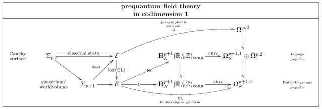
In summary then, the refinement of an Euler-Lagrange ##p##-gerbe ##\mathbf{L}## to a Lepage-##p##-gerbe ##\Theta## is given by the following diagram:

And now higher prequantum geometry bears fruit: since transgression is a natural operation, and since  the differential coefficients ##\mathbf{B}_H^{p+1}(\mathbb{R}/_{\!\hbar}\mathbb{Z})_{\mathrm{conn}}## and ##\mathbf{B}^{p+1}_L(\mathbb{R}/_{\!\hbar}\mathbb{Z})## precisely yield the coherence data to make the
local integrals over the locally defined differential forms ##L_i## and ##\Theta_i## be globally well defined, we may now hit this entire diagram with the transgression functor ##\int_{\Sigma_p} [\Sigma_p,-]## to obtain this diagram:

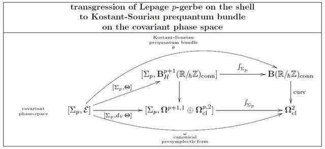
This exhibits the transgression
$$
\mathbf{\theta} := \int_{\Sigma_p} [\Sigma_p,\mathbf{\Theta}]
$$
of the Lepage ##p##-gerbe ##\mathbf{\Theta}## as a ##(\mathbb{R}/_{\!\hbar}\mathbb{Z})##-connection whose curvature is the canonical presymplectic form.

But this ##([\Sigma,\mathcal{E}]_\Sigma,\mathbf{\theta})## is just the structure that Souriau originally called and demanded as a prequantization of the (pre-)symplectic phase space ##([\Sigma,\mathcal{E}]_\Sigma,\omega)##.  Conversely, we see that the Lepage ##p##-gerbe ##\mathbf{\Theta}## is a “de-transgression” of the Kostant-Souriau prequantization of covariant phase space in codimension-1 to a higher prequantization in full codimension. In particular, the higher prequantization constituted by the Lepage ##p## gerbe constitutes a compatible choice of Kostant-Souriau prequantizations of covariant phase space for all choices of codimension-1 hypersurfaces at once. This is a genuine reflection of the fundamental locality of the field theory, even if we look at the field configurations globally over all of a (spatial) hypersurface ##\Sigma_p##.

Click For Forum Comments