Learn Propagators in Mathematical Quantum Field Theory

This is one chapter in a series on Mathematical Quantum Field Theory.

The previous chapter is 8. Phase space.

The next chapter is 10. Gauge symmetries.

9. Propagators

In this chapter we discuss the following topics:

• Background
  • Fourier analysis and Plane wave modes
  • Microlocal analysis and UV-Divergences
  • Cauchy principal values
• Propagators for the free scalar field on Minkowski spacetime
  • advanced and regarded propagators
  • causal propagator
  • Wightman propagator
  • Feynman propagator
  • singular support and wave front sets
• Propagators for the Dirac field on Minkowski spacetime

In the previous chapter we have seen the covariant phase space (prop. 8.6) of sufficiently nice Lagrangian field theories, which is the on-shell space of field histories equipped with the presymplectic form transgressed from the presymplectic current of the theory; and we have seen that in good cases this induces a bilinear pairing on sufficiently well-behaved observables, called the Poisson bracket (def. 8.14), which reflects the infinitesimal symmetries of the presymplectic current. This Poisson bracket is of central importance for passing to actual quantum field theory, since, as we will discuss in Quantization below, it is the infinitesimal approximation to the quantization of a Lagrangian field theory.

We have moreover seen that the Poisson bracket on the covariant phase space of a free field theory with Green hyperbolic equations of motion — the Peierls-Poisson bracket — is determined by the integral kernel of the causal Green function (prop. 8.7). Under the identification of linear on-shell observables with off-shell observables that are generalized solutions to the equations of motion (theorem 7.29) the convolution with this integral kernel may be understood as propagating the values of an off-shell observable through spacetime, such as to then compare it with any other observable at any spacetime point (prop. 8.7). Therefore the integral kernel of the causal Green function is also called the causal propagator (prop. 7.24).

This means that for Green hyperbolic free Lagrangian field theory the Poisson bracket, and hence the infinitesimal quantization of the theory, is all encoded in the causal propagator. Therefore here we analyze the causal propagator, as well as its variant propagators, in detail.

The main tool for these computations is Fourier analysis (reviewed below) by which field histories, observables, and propagators on Minkowski spacetime are decomposed as superpositions of plane waves of various frequencies, wave lengths and wave vector-direction. Using this, all propagators are exhibited as those superpositions of plane waves that satisfy the dispersion relation of the given equation of motion, relating plane wavefrequency to wave length.

This way the causal propagator is naturally decomposed into its contribution from positive and from negative frequencies. The positive frequency part of the causal propagator is called the Wightman propagator (def. 9.57 below). It turns out (prop. 9.60 below) that this is equivalently the sum of the causal propagator, which itself is skew-symmetric (cor. 9.53 below), with a symmetric component, or equivalently that the causal propagator is the skew-symmetrization of the Wightman propagator. After quantization of free field theory discussed further below, we will see that the Wightman propagator is equivalently the correlation function between two point-evaluation field observables (example 7.2) in a vacuum state of the field theory (a state in the sense of def. link ).

Moreover, by def. 7.18 the causal propagator also decomposes into its contributions with future and past support, given by the difference between the advanced and retarded propagators. These we analyze first, starting with prop. 9.52 below.

Combining these two decompositions of the causal propagator (positive/negative frequency as well as positive/negative time) yields one more propagator, the Feynman propagator (def. 9.61 below).

We will see below that the quantization of a free field theory is given by a “star product” (on observables) which is given by “exponentiating” these propagators. For that to make sense, certain pointwise products of these propagators, regarded as generalized functions (prop. 7.6) need to exist. But since the propagators are distributions with singularities, the existence of these products requires that certain potential “UV divergences” in their Fourier transforms (remark 9.27 below) are absent (“Hörmander’s criterion”, prop. 9.34 below). These UV divergences are captured by what is called the wave front set (def. 9.28 below).

The study of UV divergences of distributions via their wave front sets is called microlocal analysis and provides powerful tools for the understanding of quantum field theory. In particular, the propagation of singularities theorem (prop. 9.40) shows that for distributional solutions (def. 7.16) of Euler-Lagrange equations of motion, such as the propagators, their singular support propagates itself through spacetime along the wave front set.

Using this theorem we work out the wave front sets of the propagators (prop. 9.69 below). Via Hörmander’s criterion (prop. 9.34) this computation will serve to show why upon quantization the Wightman propagator replaces the causal propagator in the construction of the Wick algebra of quantum observables of the free field theory (discussed below in Free quantum fields) and the Feynman propagator similarly controls the quantum observables of the interacting quantum field theory (below in Feynman diagrams).

The following table summarizes the structure of the system of propagators. (The column “as vacuum expectation value of field operators” will be discussed further below in Free quantum fields).

propagators (i.e. integral kernels of Green functions)
for the wave operator and Klein-Gordon operator
on a globally hyperbolic spacetime such as Minkowski spacetime:

name	symbol	wave front set	as vacuum exp. value of field operators	as a product of field operators
causal propagator	$\begin{aligned}\Delta_S & = \Delta_+ – \Delta_- \end{aligned}$	$\phantom{A}\,\,\,-$	$\begin{aligned} & i \hbar \, \Delta_S(x,y) = \\ & \left\langle \;\left[\mathbf{\Phi}(x),\mathbf{\Phi}(y)\right]\; \right\rangle \end{aligned}$	Peierls-Poisson bracket
advanced propagator	$\Delta_+$		$\begin{aligned} & i \hbar \, \Delta_+(x,y) = \\ & \left\{ \array{ \left\langle \; \left[ \mathbf{\Phi}(x),\mathbf{\Phi}(y) \right] \; \right\rangle &\vert& x \geq y \\ 0 &\vert& y \geq x } \right. \end{aligned}$	future part of Peierls-Poisson bracket
retarded propagator	$\Delta_-$		$\begin{aligned} & i \hbar \, \Delta_-(x,y) = \\ & \left\{ \array{ \left\langle \; \left[\mathbf{\Phi}(x),\mathbf{\Phi}(y) \right] \; \right\rangle &\vert& y \geq x \\ 0 &\vert& x \geq y } \right. \end{aligned}$	past part of Peierls-Poisson bracket
Wightman propagator	$\begin{aligned} \Delta_H &= \tfrac{i}{2}\left( \Delta_+ – \Delta_-\right) + H\\ & = \tfrac{i}{2}\Delta_S + H \\ & = \Delta_F – i \Delta_- \end{aligned}$		$\begin{aligned} & \hbar \, \Delta_H(x,y) \\ & = \left\langle \; \mathbf{\Phi}(x) \mathbf{\Phi}(y) \; \right\rangle \\ & = \underset{ = 0 }{\underbrace{\left\langle \; : \mathbf{\Phi}(x) \mathbf{\Phi}(y) : \; \right\rangle}} \\ & \phantom{=} + \left\langle \; \left[ \mathbf{\Phi}^{(-)}(x), \mathbf{\Phi}^{(+)}(y) \right] \; \right\rangle \end{aligned}$	positivefrequency of Peierls-Poisson bracket, Wick algebra-product, 2-point function $\phantom{=}$ of vacuum state $\phantom{=}$ or generally of $\phantom{=}$ Hadamard state
Feynman propagator	$\begin{aligned}\Delta_F & = \tfrac{i}{2}\left( \Delta_+ + \Delta_- \right) + H \\ & = i \Delta_D + H \\ & = \Delta_H + i \Delta_- \end{aligned}$		$\begin{aligned} & \hbar \, \Delta_F(x,y) \\ & = \left\langle \; T\left( \; \mathbf{\Phi}(x)\mathbf{\Phi}(y) \;\right) \; \right\rangle \\ & = \left\{ \array{ \left\langle \; \mathbf{\Phi}(x)\mathbf{\Phi}(x) \; \right\rangle &\vert& x \geq y \\ \left\langle \; \mathbf{\Phi}(y) \mathbf{\Phi}(x) \; \right\rangle &\vert& y \geq x } \right.\end{aligned}$	time-ordered product

(see also Kocic’s overview: file)

Fourier analysis and plane wave modes

By definition, the equations of motion of free field theories (def. 5.25) are linear partial differential equations and hence lend themselves to harmonic analysis, where all field histories are decomposed into superpositions of plane waves via Fourier transform. Here we briefly survey the relevant definitions and facts of Fourier analysis.

In formal duality to the harmonic analysis of the field histories themselves, also the linear observables (def. 7.3) on the space of field histories, hence the distributional generalized functions (prop. 7.5) are subject to Fourier transform of distributions (def. 9.14 below).

Throughout, let $n \in \mathbb{N}$ and consider the Cartesian space $\mathbb{R}^n$ of dimension $n$ (def. 1.1). In the application to field theory, $n = p + 1$ is the dimension of spacetime and $\mathbb{R}^n$ is either Minkowski spacetime $\mathbb{R}^{p,1}$ (def. 2.17) or its wave vectors (def. 9.1 below). For $x = (x^\mu) \in \mathbb{R}^{p,1}$ and $k = (k_\mu) \in (\mathbb{R}^(p,1))^\ast$ we write

$$
x \cdot k \;=\; x^\mu k_\mu
$$

for the canonical pairing.

Definition 9.1. (plane wave)

A plane wave on Minkowski spacetime $\mathbb{R}^{p,1}$ (def. 2.17) is a smooth function with values in the complex numbers given by

$$
\array{
\mathbb{R}^{p,1} &\longrightarrow& \mathbb{C}
\\
(x^\mu) &\mapsto& e^{i k_\mu x^\mu}
}
$$

for $k = (k_\mu) \in (\mathbb{R}^{p,1})^\ast$ a covector, called the wave vector of the plane wave.

We use the following terminology:

plane waves on Minkowski spacetime

$$
\array{
\mathbb{R}^{p,1}
&\overset{\psi_k}{\longrightarrow}&
\mathbb{C}
\\
x &\mapsto& \exp\left( \, i k_\mu x^\mu \, \right)
\\
(\vec x, x^0) &\mapsto& \exp\left( \, i \vec k \cdot \vec x + i k_0 x^0 \, \right)
\\
(\vec x, c t) &\mapsto& \exp\left( \, i \vec k \cdot \vec x – i \omega t \, \right)
}
$$

symbol	name
$c$	speed of light
$\hbar$	Planck’s constant
$m$	mass
$\frac{\hbar}{m c}$	Compton wavelength
$k$, $\vec k$	wave vector
$\lambda = 2\pi/{\vert \vec k \vert}$	wave length
${\vert \vec k \vert} = 2\pi/\lambda$	wave number
$\omega := k^0 c = -k_0 c = 2\pi \nu$	angular frequency
$\nu = \omega / 2 \pi$	frequency
$p = \hbar k$, $\vec p = \hbar \vec k$	momentum
$E = \hbar \omega$	energy
	$\omega(\vec k) = c \sqrt{ \vec k^2 + \left(\frac{m c}{\hbar}\right)^2 }$	Klein-Gordon dispersion relation
$E(\vec p) = \sqrt{ c^2 \vec p^2 + (m c^2)^2 }$	energy-momentum relation

Definition 9.2. (Schwartz space of functions with rapidly decreasing partial derivatives)

A complex-valued smooth function $f \in C^\infty(\mathbb{R}^n)$ is said to have rapidly decreasing partial derivatives if for all $\alpha,\beta \in \mathbb{N}^{n}$ we have

$$
\underset{x \in \mathbb{R}^n}{sup} {\vert x^\beta \partial^\alpha f(x) \vert}
\;\lt\; \infty
\,.
$$

Write

$$
\mathcal{S}(\mathbb{R}^n) \hookrightarrow C^\infty(\mathbb{R}^n)
$$

for the sub-vector space on the functions with rapidly decreasing partial derivatives regarded as a topological vector space for the Fréchet space structure induced by the seminorms

$$
p_{\alpha, \beta}(f) := \underset{x \in \mathbb{R}^n}{sup} {\vert x^\beta \partial^\alpha f(x) \vert}
\,.
$$

This is also called the Schwartz space.

(e.g. Hörmander 90, def. 7.1.2)

Example 9.3. (compactly supported smooth function are functions with rapidly decreasing partial derivatives)

Every compactly supported smooth function (bump function) $b \in C^\infty_{cp}(\mathbb{R}^n)$ has rapidly decreasing partial derivatives (def. 9.2):

$$
C^\infty(\mathbb{R}^n)
\hookrightarrow
\mathcal{S}(\mathbb{R}^n)
\,.
$$

Proposition 9.4. (pointwise product and convolution product on Schwartz space)

The Schwartz space $\mathcal{S}(\mathbb{R}^n)$ (def. 9.2) is closed under the following operatios on smooth functions $f,g \in \mathcal{S}(\mathbb{R}^n) \hookrightarrow C^\infty(\mathbb{R}^n)$

1. pointwise product:$$
   (f \cdot g)(x) := f(x) \cdot g(x)
   $$
2. convolution product:$$
   (f \star g)(x) := \underset{y \in \mathbb{R}^n}{\int} f(y)\cdot g(x-y) \, dvol(y)
   \,.
   $$

Proof. By the product law of differentiation>.

Proposition 9.5. (rapidly decreasing functions are integrable)

Every rapidly decreasing function $f \colon \mathbb{R}^n \to \mathbb{R}$ (def. 9.2) is an integrable function in that its integral exists:

$$
\underset{x \in \mathbb{R}^n}{\int} f(x) \, d^n x
\;\lt\;
\infty
$$

In fact for each $\alpha \in \mathbb{N}^n$ the product of $f$ with the $\alpha$-power of the coordinate functions exists:

$$
\underset{x \in \mathbb{R}^n}{\int}
x^\alpha f(x)\, d^n x
\;\lt\;
\infty
\,.
$$

Definition 9.6. (Fourier transform of functions with rapidly decreasing partial derivatives)

The Fourier transform is the continuous linear functional

$$
\widehat{(-)}
\;\colon\;
\mathcal{S}(\mathbb{R}^n)
\longrightarrow
\mathcal{S}(\mathbb{R}^n)
$$

on the Schwartz space of functions with rapidly decreasing partial derivatives (def. 9.2), which is given by integration against plane wave functions (def. 9.1)

$$
x \mapsto e^{- i k \cdot x}
$$

times the standard volume form $d^n x$:

$$
\label{IntegralExpressionForFourierTransform}
\hat f(k)
\;\colon\;
\int_{x \in \mathbb{R}^n}
e^{- i \, k \cdot x} f(x) \, d^n x
\,.
$$ (123)

Here the argument $k \in \mathbb{R}^n$ of the Fourier transform is also called the wave vector.

(e.g. Hörmander, lemma 7.1.3)

Proposition 9.7. (Fourier inversion theorem)

The Fourier transform $\widehat{(-)}$ (def. 9.6) on the Schwartz space $\mathcal{S}(\mathbb{R}^n)$ (def. 9.2) is an isomorphism, with inverse function the inverse Fourier transform

$$
\widecheck {(-)}
\;\colon\;
\mathcal{S}(\mathbb{R}^n) \longrightarrow \mathcal{S}(\mathcal{R}^n)
$$

given by

$$
\widecheck g (x)
\;:=\;
\underset{k \in \mathbb{R}^n}{\int}
g(k) e^{i k \cdot x}
\, \frac{d^n k}{(2\pi)^n}
\,.
$$

Hence in the language of harmonic analysis, the function $\widecheck g \colon \mathbb{R}^n \to \mathbb{C}$ is the superposition of plane waves (def. 9.1) in which the plane wave with wave vector $k\in \mathbb{R}^n$ appears with amplitude $g(k)$.

(e.g. Hörmander, theorem 7.1.5)

Proposition 9.8. (basic properties of the Fourier transform)

The Fourier transform $\widehat{(-)}$ (def. 9.6) on the Schwartz space $\mathcal{S}(\mathbb{R}^n)$ (def. 9.2) satisfies the following properties, for all $f,g \in \mathcal{S}(\mathbb{R}^n)$:

1. (interchanging coordinate multiplication with partial derivatives)
   

   $$
   \label{FourierTransformInterchangesCoordinateProductWithDerivative}
   \widehat{ x^a f } = + i \partial_a \widehat f
   \phantom{AAAAA}
   \widehat{ – i\partial_a f} = k_a \widehat f
   $$ (124)

2. (interchanging pointwise multiplication with convolution product, remark 9.4):
   

   $$
   \label{FourierTransformInterchangesPointwiseProductWithConvolution}
   \widehat {(f \star g)} = \widehat{f} \cdot \widehat{g}
   \phantom{AAAA}
   \widehat{ f \cdot g } = (2\pi)^{-n} \widehat{f} \star \widehat{g}
   $$ (125)

3. (unitarity, Parseval’s theorem)$$
   \underset{x \in \mathbb{R}^n}{\int} f(x) g^\ast(x)\, d^n x
   \;=\;
   \underset{k \in \mathbb{R}^n}{\int} \widehat{f}(k) \widehat{g}^\ast(k) \, d^n k
   $$

4. $$
   \label{FourierTransformInIntegralOfProductMayBeShiftedToOtherFactor}
   \underset{k \in \mathbb{R}^n}{\int} \widehat{f}(k) \cdot g(k) \, d^n k
   \;=\;
   \underset{x \in \mathbb{R}^n}{\int} f(x) \cdot \widehat{g}(x) \, d^n x
   $$ (126)

(e.g Hörmander 90, lemma 7.1.3, theorem 7.1.6)

The Schwartz space of functions with rapidly decreasing partial derivatives (def. 9.2) serves the purpose to support the Fourier transform (def. 9.6) together with its inverse (prop. 9.7), but for many applications, one needs to apply the Fourier transform to more general functions and in fact to generalized functions in the sense of distributions (via this prop.). But with the Schwartz space in hand, this generalization is readily obtained by formal duality:

Definition 9.9. (tempered distribution)

A tempered distribution is a continuous linear functional

$$
u \;\colon\; \mathcal{S}(\mathbb{R}^n) \longrightarrow \mathbb{C}
$$

on the Schwartz space (def. 9.2) of functions with rapidly decaying partial derivatives. The vector space of all tempered distributions is canonically a topological vector space as the dual space to the Schwartz space, denoted

$$
\mathcal{S}'(\mathbb{R}^n)
\;:=\;
\left(
\mathcal{S}(\mathbb{R}^n)
\right)^\ast
\,.
$$

e.g. (Hörmander 90, def. 7.1.7)

Example 9.10. (some non-singular tempered distributions)

Every function with rapidly decreasing partial derivatives $f \in \mathcal{S}(\mathbb{R}^n)$ (def. 9.2) induces a tempered distribution $u_f \in \mathcal{S}'(\mathbb{R}^n)$ (def. 9.9) by integrating against it:

$$
u_f \;\colon\; g \mapsto \underset{x \in \mathbb{R}^n}{\int} g(x) f(x)\, d^n x
\,.
$$

This construction is a linear inclusion

$$
\mathcal{S}(\mathbb{R}^n) \overset{\text{dense}}{\hookrightarrow} \mathcal{S}'(\mathbb{R}^n)
$$

of the Schwartz space into its dual space of tempered distributions. This is a dense subspace inclusion.

In fact already the restriction of this inclusion to the compactly supported smooth functions (example 9.3) is a dense subspace inclusion:

$$
C^\infty_{cp}(\mathbb{R}^n)
\overset{dense}{\hookrightarrow}
\mathcal{S}'(\mathbb{R}^n)
\,.
$$

This means that every tempered distribution is a limit of a sequence of ordinary functions with rapidly decreasing partial derivatives and in fact even the limit of a sequence of compactly supported smooth functions (bump functions).

It is in this sense that tempered distributions are “generalized functions”.

(e.g. Hörmander 90, lemma 7.1.8)

Example 9.11. (compactly supported distributions are tempered distributions)

Every compactly supported distribution is a tempered distribution (def. 9.9), hence there is a linear inclusion

$$
\mathcal{E}'(\mathbb{R}^n)
\hookrightarrow
\mathcal{S}'(\mathbb{R}^n)
\,.
$$

Example 9.12. (delta distribution)

Write

$$
\delta_0(-) \;\in\; \mathcal{E}'(\mathbb{R}^n)
$$

for the distribution given by point evaluation of functions at the origin of $\mathbb{R}^n$:

$$
\delta_0(-) \;\colon\; f \mapsto f(0)
\,.
$$

This is clearly a compactly supported distribution; hence a tempered distribution by example 9.11.

We write just “$\delta(-)$” (without the subscript) for the corresponding generalized function (example 9.10), so that

$$
\underset{x \in \mathbb{R}^n}{\int} \delta(x) f(x) \, d^n x
\;:=\;
f(0)
\,.
$$

Example 9.13. (square integrable functions induce tempered distributions)

Let $f \in L^p(\mathbb{R}^n)$ be a function in the $p$th Lebesgue space, e.g. for $p = 2$ this means that $f$ is a square integrable function. Then the operation of integration against the measure $f dvol$

$$
g \mapsto \underset{x \in \mathbb{R}^n}{\int} g(x) f(x) \, d^n x
$$

is a tempered distribution (def. 9.9).

(e.g. Hörmander 90, below lemma 7.1.8)

Property (126) of the ordinary Fourier transform on functions with rapidly decreasing partial derivatives motivates and justifies the following generalization:

Definition 9.14. (Fourier transform of distributions on tempered distributions)

The Fourier transform of distributions of a tempered distribution $u \in \mathcal{S}'(\mathbb{R}^n)$ (def. 9.9) is the tempered distribution $\widehat u$ defined on a smooth function $f \in \mathcal{S}(\mathbb{R}^n)$ in the Schwartz space (def. 9.2) by

$$
\widehat{u}(f) \;:=\; u\left( \widehat f\right)
\,,
$$

where on the right $\widehat f \in \mathcal{S}(\mathbb{R}^n)$ is the Fourier transform of functions from def. 9.6.

(e.g. Hörmander 90, def. 1.7.9)

Example 9.15. (Fourier transform of distributions indeed generalizes Fourier transform of functions with rapidly decreasing partial derivatives)

Let $u_f \in \mathcal{S}'(\mathbb{R}^n)$ be a non-singular tempered distribution induced, via example 9.10, from a function with rapidly decreasing partial derivatives $f \in \mathcal{S}(\mathbb{R}^n)$.

Then its Fourier transform of distributions (def. 9.14) is the non-singular distribution induced from the Fourier transform of $f$:

$$
\widehat{u_f} \;=\; u_{\hat f}
\,.
$$

Proof. Let $g \in \mathcal{S}(\mathbb{R}^n)$. Then

$$
\begin{aligned}
\widehat{u_f}(g)
& :=
u_f\left( \widehat{g}\right)
\\
& =
\underset{x \in \mathbb{R}^n}{\int} f(x) \hat g(x)\, d^n x
\\
& =
\underset{x \in \mathbb{R}^n}{\int} \hat f(x) g(x) \, d^n x
\\
& =
u_{\hat f}(g)
\end{aligned}
$$

Here all equalities hold by definition, except for the third: this is property (126) from prop. 9.8.

Example 9.16. (Fourier transform of Klein-Gordon equation of distributions)

Let $\Delta \in \mathcal{S}'(\mathbb{R}^{p,1})$ be any tempered distribution (def. 9.9) on Minkowski spacetime (def. 2.17) and let $P := \eta^{\mu \nu} \frac{\partial}{\partial x^\mu}\frac{\partial}{\partial x^\nu} – \left( \tfrac{m c}{\hbar} \right)^2$ be the Klein-Gordon operator (68). Then the Fourier transform (def. 9.14) of $P \Delta$ is, in generalized function-notation (remark 7.7)given by

$$
\widehat {P \Delta}(k)
\;=\;
\left(
– \eta^{\mu \nu}k_\mu k_\nu
– \left( \tfrac{m c}{\hbar}\right)^2
\right)
\widehat(k)
\,.
$$

Proof. Let $r \in \mathcal{S}(\mathbb{R}^n)$ be any function with rapidly decreasing partial derivatives (def. 9.2). Then

$$
\begin{aligned}
\widehat {P \Delta}(r)
& =
P \Delta(\widehat r)
\\
& =
\Delta(P^\ast \widehat r)
\\
& =
\Delta(P \widehat r)
\\
& =
\Delta\left( \left(-\eta^{\mu \nu}k_\mu k_\nu – \left( \tfrac{m c}{\hbar}\right)^2\right) \widehat{r} \right)
\end{aligned}
$$

Here the first step is def. 9.14, the second is def. 7.16, the third is example 5.28, while the last step is prop. 9.8.

Example 9.17. (Fourier transform of compactly supported distributions)

Under the identification of smooth functions of bounded growth with non-singular tempered distributions (example 9.10), the Fourier transform of distributions (def. 9.14) of a tempered distribution that happens to be compactly supported (example 9.11)

$$
u \in \mathcal{E}'(\mathbb{R}^n) \hookrightarrow \mathcal{S}'(\mathbb{R}^n)
$$

is simply

$$
\widehat{u}(k) = u\left( e^{- i k \cdot (-)}\right)
\,.
$$

(Hörmander 90, theorem 7.1.14)

Example 9.18. (Fourier transform of the delta-distribution)

The Fourier transform (def. 9.14) of the delta distribution (def. 9.12), via example 9.17, is the constant function on 1:

$$
\begin{aligned}
\widehat {\delta}(k)
& =
\underset{x \in \mathbb{R}^n}{\int} \delta(x) e^{- i k x} \, d x
\\
& =
1
\end{aligned}
$$

This implies by the Fourier inversion theorem (prop. 9.20) that the delta distribution itself has equivalently the following expression as a generalized function

$$
\begin{aligned}
\delta(x)
& =
\widecheck{\widehat {\delta_0}}(x)
\\
& =
\underset{k \in \mathbb{R}^n}{\int} e^{i k \cdot x} \, \frac{d^n k}{ (2\pi)^n }
\end{aligned}
$$

in the sense that for every function with rapidly decreasing partial derivatives $f \in \mathcal{S}(\mathbb{R}^n)$ (def. 9.2) we have

$$
\begin{aligned}
f(x)
& =
\underset{y \in \mathbb{R}^n}{\int}
f(y) \delta(y-x) \, d^n y
\\
& =
\underset{y \in \mathbb{R}^n}{\int}
\underset{k \in \mathbb{R}^n}{\int}
f(y) e^{i k \cdot (y-x)}
\, \frac{d^n k}{(2\pi)^n} \, d^n y
\\
& =
\underset{k \in \mathbb{R}^n}{\int}
e^{- i k \cdot x}
\underset{= \widehat{f}(-k) }{
\underbrace{
\underset{y \in \mathbb{R}^n}{\int}
f(y) e^{i k \cdot y}
\, d^n y
}
}
\,\, \frac{d^n k}{(2\pi)^n}
\\
& =
+
\underset{k \in \mathbb{R}^n}{\int}
e^{i k \cdot x}
\underset{= \widehat{f}(k) }{
\underbrace{
\underset{y \in \mathbb{R}^n}{\int}
f(y) e^{- i k \cdot y}
\, d^n y
}
}
\,\, \frac{d^n k}{(2\pi)^n}
\\
& =
\widecheck{\widehat{f}}(x)
\end{aligned}
$$

which is the statement of the Fourier inversion theorem for smooth functions (prop. 9.7).

(Here in the last step we used the change of integration variables $k \mapsto -k$ which introduces one sign $(-1)^{n}$ for the new volume form, but another sign $(-1)^n$ from the re-orientation of the integration domain. )

Equivalently, the above computation shows that the delta distribution is the neutral element for the convolution product of distributions.

Proposition 9.19. (Paley-Wiener-Schwartz theorem I)

Let $u \in \mathcal{E}'(\mathbb{R}^n) \hookrightarrow \mathcal{S}'(\mathbb{R}^n)$ be a compactly supported distribution regarded as a tempered distribution by example 9.11. Then its Fourier transform of distributions (def. 9.14) is a non-singular distribution induced from a smooth function that grows at most exponentially.

(e.g. Hoermander 90, theorem 7.3.1)

Proposition 9.20. (Fourier inversion theorem for Fourier transform of distributions)

The operation of forming the Fourier transform of distributions $\widehat{u}$ (def. 9.14) tempered distributions $u \in \mathcal{S}'(\mathbb{R}^n)$ (def. 9.9) is an isomorphism, with inverse given by

$$
\widecheck{ u } \;\colon\; g \mapsto u\left( \widecheck{g}\right)
\,,
$$

where on the right $\widecheck{g}$ is the ordinary inverse Fourier transform of $g$ according to prop. 9.7.

Proof. By def. 9.14
this follows immediately from the Fourier inversion theorem for smooth functions (prop. 9.7).

We have the following distributional generalization of the basic property (125) from prop. 9.8:

Proposition 9.21. (Fourier transform of distributions interchanges convolution of distributions with pointwise product)

Let

$$
u_1 \in \mathcal{S}'(\mathbb{R}^n)
$$

be a tempered distribution (def. 9.9) and

$$
u_2 \in \mathcal{E}'(\mathbb{R}^n) \hookrightarrow \mathcal{S}'(\mathbb{R}^n)
$$

be a compactly supported distribution, regarded as a tempered distribution via example 9.11.

Observe here that the Paley-Wiener-Schwartz theorem (prop. 9.19) implies that the Fourier transform of distributions of $u_1$ is a non-singular distribution $\widehat{u_1} \in C^\infty(\mathbb{R}^n)$ so that the product $\widehat{u_1} \cdot \widehat{u_2}$ is always defined.

Then the Fourier transform of distributions of the convolution product of distributions is the product of the Fourier transform of distributions:

$$
\widehat{u_1 \star u_2}
\;=\;
\widehat{u_1} \cdot \widehat{u_2}
\,.
$$

(e.g. Hörmander 90, theorem 7.1.15)

Remark 9.22. (product of distributions via Fourier transform of distributions)

Prop. 9.21 together with the Fourier inversion theorem (prop. 9.20) suggests to define the product of distributions $u_1 \cdot u_2$ for compactly supported distributions $u_1, u_2 \in \mathcal{E}'(\mathbb{R}^n) \hookrightarrow \mathcal{S}'(\mathbb{R}^n)$ by the formula

$$
\widehat{ u_1 \cdot u_2 }
\;:=\;
(2\pi)^n \widehat{u_1} \star \widehat{u_2}
$$

which would complete the generalization of of property (125) from prop. 9.8.

For this to make sense, the convolution product of the smooth functions on the right needs to exist, which is not guaranteed (prop. 9.4 does not apply here!). The condition that this exists is the Hörmander criterion on the wave front set (def. 9.28) of $u_1$ and $u_2$ (prop. 9.34 belwo). This we further discuss in Microlocal analysis and UV-Divergences below.

microlocal analysis and ultraviolet divergences

A distribution (def. 7.5) or generalized function (prop. 7.6) is like a smooth function that may have “singularities”, namely points at which it values or that of its derivatives “become infinite”. Conversely, smooth functions are the non-singular distributions (prop. 7.6). The collection of points around which a distribution is singular (i.e. not non-singular) is called its singular support (def. 9.24 below).

The Fourier transform of distributions (def. 9.14) decomposes a generalized function into the plane wave modes that it is made of (def. 9.1). The Paley-Wiener-Schwartz theorem (prop. 9.26 below) says that the singular nature of a compactly supported distribution may be read off from this Fourier mode decomposition: Singularities correspond to large contributions by Fourier modes of highfrequency and small wavelength, hence to large “ultraviolet” (UV) contributions (remark 9.27 below). Therefore the singular support of a distribution is the set of points around which the Fourier transform does not sufficiently decay “in the UV”.

But since the Fourier transform is a function of the full wave vector of the plane wave modes (def. 9.1), not just of thefrequency/wavelength, but also of the direction of the wave vector, this means that it contains directional information about the singularities: A distribution may have UV-singularities at some point and in some wave vector direction, but maybe not in other directions.

In particular, if the distribution in question is a distributional solution to a partial differential equation (def. 7.16) on spacetime then the propagation of singularities theorem (prop. 9.40 below) says that the singular support of the solution evolves in spacetime along the direction of those wave vectors in which the Fourier transform exhibits high UV constributions. This means that these directions are the “wave front” of the distributional solution. Accordingly, the singular support of a distribution together with, over each of its points, the directions of wave vectors in which the Fourier transform around that point has large UV constributions is called the wave front set of the distribution (def. 9.28 below).

What is called microlocal analysis is essentially the analysis of distributions with attention to their wave front set, hence to the wave vector-directions of UV divergences.

In particular the product of distributions is well defined (only) if the wave front sets of the distributions to not “collide”. And this in fact motivates the definition of the wave front set:

To see this, let $u,v \in \mathcal{D}'(\mathbb{R}^1)$ be two distributions, for simplicity of exposition taken on the real line.

Since the product $u \cdot v$, is, if it exists, supposed to generalize the pointwise product of smooth functions, it must be fixed locally: for every point $x \in \mathbb{R}$ there ought to be a compactly supported smooth function (bump function) $b \in C^\infty_{cp}(\mathbb{R})$ with $f(x) = 1$ such that

$$
b^2 u \cdot v = (b u) \cdot (b v)
\,.
$$

But now $b v$ and $b u$ are both compactly supported distributions (def. 9.25 below), and these have the special property that their Fourier transforms $\widehat{b v}$ and $\widehat{b u}$ are, in particular, smooth functions (by the Paley-Wiener-Schwartz theorem, prop 9.19).

Moreover, the operation of Fourier transform interchanges pointwise products with convolution products (prop. 9.8). This means that if the product of distributions $u \cdot v$ exists, it must locally be given by the inverse Fourier transform of the convolution product of the Fourier transforms $\widehat {b u}$ and $\widehat b v$:

$$
\widehat{ b^2 u \cdot v }(x)
\;=\;
\underset{\underset{k_{max} \to \infty}{\longrightarrow}}{\lim}
\,
\int_{- k_{max}}^{k_{max}} \widehat{(b u)}(k) \widehat{(b v)}(x – k) d k
\,.
$$

(Notice that the converse of this formula holds as a fact by prop. 9.21)

This shows that the product of distributions exists once there is a bump function $b$ such that the integral on the right converges as $k_{max} \to \infty$.

Now the Paley-Wiener-Schwartz theorem says more, it says that the Fourier transforms $\widehat {b u}$ and $\widehat {b u}$ are polynomially bounded. On the other hand, the integral above is well defined if the integrand decreases at least quadratically with $k \to \infty$. This means that for the convolution product to be well defined, either $\widehat {b u}$ has to polynomially decrease faster with $k \to \pm \infty$ than $\widehat {b v}$ grows in the other direction, $k \to \mp \infty$ (due to the minus sign in the argument of the second factor in the convolution product), or the other way around.

Moreover, the degree of polynomial growth of the Fourier transform increases by one with each derivative (def. 7.16). Therefore if the product law for derivatives of distributions is to hold generally, we need that either $\widehat{b u}$ or $\widehat{b v}$ decays faster than any polynomial in the opposite of the directions in which the respective other factor does not decay.

Here the set of directions of wave vectors in which the Fourier transform of a distribution localized around any point does not decay exponentially is the wave front set of a distribution (def. 9.28 below). Hence the condition that the product of two distributions is well defined is that for each wave vector direction in the wave front set of one of the two distributions, the opposite direction must not be an element of the wave front set of the other distribution. This is called Hörmander’s criterion (prop. 9.34 below).

We now say this in detail:

Definition 9.23. (restriction of distributions)

For $U \subset \mathbb{R}^n$ a subset, and $u \in \mathcal{D}'(\mathbb{R}^n)$ a distribution, then the restriction of $u$ to $U$ is the distribution

$$
u\vert_U \in \mathcal{D}'(U)
$$

give by restricting $u$ to test functions whose support is in $U$.

Definition 9.24. (singular support of a distribution)

Given a distribution $u \in \mathcal{D}'(\mathbb{R}^n)$, a point $x \in \mathbb{R}^n$ is a singular point if there is no neighbourhood $U \subset \mathbb{R}^n$ of $x$ such that the restriction $u\vert_U$ (def. 9.23) is a non-singular distribution (given by a smooth function).

The set of all singular points is the singular support $supp_{sing}(u) \subset \mathbb{R}^n$ of $u$.

Definition 9.25. (product of a distribution with a smooth function)

Let $u \in \mathcal{D}'(\mathbb{R}^n)$ be a distribution, and $f \in C^\infty(\mathbb{R}^n)$ a smooth function. Then the product $f u \in \mathcal{D}'(\mathbb{R}^n)$ is the evident distribution given on a test function $b \in C^\infty_{cp}(\mathbb{R}^n)$ by

$$
f u
\;\colon\;
u
\mapsto
u(f \cdot b)
\,
$$

Proposition 9.26. (Paley-Wiener-Schwartz theorem II — decay of Fourier transform of compactly supported functions)

A compactly supported distribution $u \in \mathcal{E}'(\mathbb{R}^n)$ is non-singular, hence given by a compactly supported function $b \in C^\infty_{cp}(\mathbb{R}^n)$ via $u(f) = \int b(x) f(x) dvol(x)$, precisely if its Fourier transform $\hat u$ (this def.) satisfies the following decay property:

For all $N \in \mathbb{N}$ there exists $C_N \in \mathbb{R}_+$ such that for all $k \in \mathbb{R}^n$ we have that the absolute value ${\vert \hat v(k)\vert}$ of the Fourier transform at that point is bounded by

$$
\label{DecayEstimateForFourierTransformOfNonSingularDistribution}
{\vert \hat v(k)\vert}
\;\leq\;
C_N \left( 1 + {\vert k\vert} \right)^{-N}
\,.
$$ (127)

(Hörmander 90, around (8.1.1))

Remark 9.27. (ultraviolet divergences)

In other words, the Paley-Wiener-Schwartz theorem II (prop. 9.26) says that the singularities of a distribution “in position space” are reflected in non-decaying contributions of high frequencies (small wavelength) in its Fourier mode-decomposition (def. 9.14). Since for ordinary light waves one associates highfrequency with the “ultraviolet”, we may think of these as “ultaviolet contributions”.

But apart from the wavelength, the wave vector that the Fourier transform of distributions depends on also encodes the direction of the corresponding plane wave. Therefore the Paley-Wiener-Schwartz theorem says in more detail that a distribution is singular at some point already if along any one direction of the wave vector its local Fourier transform picks up ultraviolet contributions in that direction.

It, therefore, makes sense to record this extra directional information in the singularity structure of a distribution. This is called the wave front set (def. 9.28) below. The refined study of singularities taking this directional information into account is what is called microlocal analysis.

Moreover, the Paley-Wiener-Schwartz theorem I (prop. 9.19) says that if the ultraviolet contributions diverge more than polynomially with highfrequency, then the corresponding would-be compactly supported distribution is not only singular, but is actually ill-defined.

Such ultraviolet divergences appear notably when forming a would-be product of distributions whose two factors have wave front sets whose UV-contributions “add up”. This condition for the appearance/avoidance of UV-divergences is called Hörmander’s criterion (prop. 9.34 below).

Definition 9.28. (wavefront set)

Let $u \in \mathcal{D}'(\mathbb{R}^n)$ be a distribution. For $b \in C^\infty_{cp}(\mathbb{R}^n)$ a compactly supported smooth function, write $b u \in \mathcal{E}'(\mathbb{R}^n)$ for the corresponding product (def. 9.25), which is now a compactly supported distribution.

For $x\in supp(b) \subset \mathbb{R}^n$, we say that a unit covector $k \in S((\mathbb{R}^n)^\ast)$ is regular if there exists a neighbourhood $U \subset S((\mathbb{R}^n)^\ast)$ of $k$ in the unit sphere such that for all $c k’ \in (\mathbb{R}^n)^\ast$ with $c \in \mathbb{R}_+$ and $k’ \in U \subset S((\mathbb{R}^n)^\ast)$ the decay estimate (127) is valid for the Fourier transform $\widehat{b u}$ of $b u$; at $c k’$. Otherwise $k$ is non-regular. Write

$$
\Sigma(b u)
\;:=\;
\left\{
k \in S((\mathbb{R}^n)^\ast)
\;\vert\;
k \, \text{non-regular}
\right\}
$$

for the set of non-regular covectors of $b u$.

The wave front set at $x$ is the intersection of these sets as $b$ ranges over bump functions whose support includes $x$:

$$
\Sigma_x(u)
\;:=\;
\underset{
{ b \in C^\infty_{cp}(\mathbb{R}^n) }
\atop
{ x \in supp(b) }
}{\cap}
\Sigma(b u)
\,.
$$

Finally the wave front set of $u$ is the subset of the sphere bundle $S(T^\ast \mathbb{R}^n)$ which over $x \in \mathbb{R}^n$ consists of $\Sigma_x(U) \subset T^\ast_x \mathbb{R}^n$:

$$
WF(u)
\;:=\;
\underset{x \in \mathbb{R}^n}{\cup}
\Sigma_x(u)
\;\subset\;
S(T^\ast \mathbb{R}^n)
$$

Often this is equivalently considered as the full conical set inside the cotangent bundle generated by the unit covectors under multiplication with positive real numbers.

(Hörmander 90, def. 8.1.2)

Remark 9.29. (wave front set is the UV divergence-direction-bundle over the singular support)

For $u \in \mathcal{D}'(\mathbb{R}^n)$ The Paley-Wiener-Schwartz theorem (prop. 9.26) implies that

1. Forgetting the direction covectors in the wave front set $WF(u)$ (def. 9.28) and remembering only the points where they are based yields the set of singulars points of $u$, hence the singular support (def. 9.24)$$
   \array{
   WF(u)
   \\
   \downarrow
   \\
   supp_{sing}(u) &\hookrightarrow& \mathbb{R}^n
   }
   $$
2. the wave front set is empty, precisely if the singular support is empty, which is the case precisely if $u$ is a non-singular distribution.

Example 9.30. (wave front set of non-singular distribution is empty)

By prop. 9.26, the wave front set (def. 9.29) of a non-singular distribution (prop. 7.6) is empty. Conversely, a distribution is non-singular if its wave front set is empty:

$$
u \in \mathcal{D}’\;\text{non-singular}
\phantom{AA}
\Leftrightarrow
\phantom{AA}
WF(u) = \emptyset
$$

Example 9.31. (wave front set of delta distribution)

Consider the delta distribution

$$
\delta_0 \in \mathcal{D}'(\mathbb{R}^n)
$$

given by evaluation at the origin. Its wave front set (def. 9.28) consists of all the directions at the origin:

$$
WF(\delta_0)
\;=\;
\left\{
(0,k)
\;\vert\;
k \in \mathbb{R}^n \setminus \{0\}
\right\}
\subset
\mathbb{R}^n \times \mathbb{R}^n
\simeq
T^\ast \mathbb{R}^n
\,.
$$

Proof. First of all the singular support (def. 9.24) of $\delta_0$ is clearly $supp_{sing}(\delta(0)) = \{0\}$, hence by remark 9.29 the wave front set vanishes over $\mathbb{R}^n \setminus \{0\}$.

At the origin, any bump function $b$ supported around the origin with $b(0) = 1$ satisfies $b \cdot \delta(0) = \delta(0)$ and hence the wave front set over the origin is the set of covectors along which the Fourier transform $\hat \delta(0)$ does not suitably decay. But this Fourier transform is in fact a constant functionS (example 9.18) and hence does not decay in any direction.

Example 9.32. (wave front set of step function)

Let $\Theta \in \mathcal{D}'(\mathbb{R}^1)$ be the Heaviside step function given by

$$
\Theta(b) := \int_0^\infty b(x)\, d x
\,.
$$

Its wave front set (def. 9.28) is

$$
WF(H) = \{(0,k) \vert k \neq 0\}
\,.
$$

Proposition 9.33. (wave front set of convolution of compactly supported distributions)

Let $u,v \in \mathcal{E}'(\mathbb{R}^n)$ be two compactly supported distributions. Then the wave front set (def. 9.28) of their convolution of distributions (def. link ) is

$$
WF(u \star v)
\;=\;
\left\{
(x + y, k)
\;\vert\;
(x,k) \in WF(u) \,\text{and}\, (y,k) \in WF(u)
\right\}
\,.
$$

(Bengel 77, prop. 3.1)

Proposition 9.34. (Hörmander’s criterion for product of distributions)

Let $u, v \in \mathcal{D}'(\mathbb{R}^n)$ be two distributions. If their wave front sets (def 9.28) do not collide, in that for $v \in T^\ast_x X$ a covector contained in one of the two wave front sets then the covector $-v \in T^\ast_x X$ with the opposite direction in not contained in the other wave front set, i.e. the intersection fiber product inside the cotangent bundle $T^\ast X$ of the pointwise sum of wave fronts with the zero sectionis empty:

$$
\left( WF(u_1) + WF(u_2) \right) \underset{T^\ast X}{\times} X
\;=\;
\emptyset
$$

i.e.

$$
\array{
&& \emptyset
\\
& \swarrow && \searrow
\\
WF(u_1) + WF(u_2) && (pb) && X
\\
& \searrow && \swarrow_{\rlap{0}}
\\
&& T^\ast X
}
$$

then the product of distributions $u \cdot v$ exists, given, locally, by the Fourier inversion of the convolution product of their Fourier transform of distributions (remark 9.22).

For making use of wave front sets, we need a collection of results about how wave front sets change as we apply certain operations to distributions:

Proposition 9.35. (differential operator preserves or shrinks wave front set)

Let $P$ be a differential operator (def. 4.7). Then for $u \in \mathcal{D}’$ a distribution, the wave front set (def. 9.28) of the derivative of distributions $P u$ (def. 7.16) is contained in the original wave front set of $u$:

$$
WF(P u) \subset WF(u)
$$

(Hörmander 90, (8.1.11))

Proposition 9.36. (wave front set of product of distributions is inside fiber-wise sum of wave front sets)

Let $u,v \in \mathcal{D}'(X)$ be a pair of distributions satisfying Hörmander’s criterion, so that their product of distributions $u \cdot v$ exists by prop. 9.34. Then the wave front set (def. 9.28) of the product distribution is contained inside the fiber-wise sum of the wave front set elements of the two factors:

$$
WF(u \cdot v)
\;\subset\;
(WF(u) \cup (X \times \{0\}))
+
(WF(v) \cup (X \times \{0\}))
\,.
$$

(Hörmander 90, theorem 8.2.10)

More generally:

Proposition 9.37. (partial product of distributions of several variables)

Let

$$
K_1 \in \mathcal{D}'(X \times Y)
\phantom{AAA}
K_2 \in \mathcal{D}'(Y \times Z)
$$

be two distributions of two variables. For their product of distributions to be defined over $Y$, Hörmander’s criterion on the pair of wave front sets $WF(K_1), WF(K_2)$ needs to hold for the wave front wave vectors along $X$ and $Y$ taken to be zero.

If this is satisfied, then the Scomposition of integral kernels (if it exists)

$$
(K_1 \circ K_2)(-,-)
\;:=\;
\underset{Y}{\int}
K_1(-,y) K_2(y,-)
dvol_Y(y)
\;\in\;
\mathcal{D}'(X \times Z)
$$

has wave front set constrained by

$$
\label{CompositionOfIntegralKernelsWaveFronConstraint}
WF(K_1 \circ K_2)
\;\subset\;
\left\{
(x,z, k_x, k_z)
\;\vert\;
\array{
\left(
(x,y,k_x,-k_y) \in WF(K_1)
\,\,
\text{and}
\,\,
(y,z,k_y, k_z) \in WF(K_2)
\right)
\\
\text{or}
\\
\left(
k_x = 0
\,\text{and}\,
(y,z,0,-k_z) \in WF(K_2)
\right)
\\
\text{or}
\\
\left(
k_z = 0
\,\text{and}\,
(x,y,k_x,0) \in WF(K_1)
\right)
}
\right\}
$$ (128)

(Hörmander 90, theorem 8.2.14)

A key fact for identifying wave front sets is the propagation of singularities theoremS (prop. 9.40 below). In order to state this we need the following concepts regarding symbols of differential operators:

Definition 9.38. (symbol of a differential operator)

Let

$$
D
\;=\;
\underset{n \leq N}{\sum}
D^{\mu_1 \cdots \mu_n}
\frac{\partial}{\partial x^{\mu^1}}
\cdots
\frac{\partial}{\partial x^{\mu^n}}
+
D^0
$$

be a differential operator on $\mathbb{R}^n$ (def. 4.7). Then its symbol of a differential operator is the smooth function on the cotangent bundle $T^\ast \mathbb{R}^n \simeq \mathbb{R}^n \times \mathbb{R}^n$ (def. 1.12) given by

$$
\array{
T^\ast \mathbb{R}^n
&\overset{q}{\longrightarrow}&
\mathbb{C}
\\
k &\mapsto&
\underset{n \leq N}{\sum}
D^{\mu_1 \cdots \mu_k} k_{\mu_1} \cdots k_{\mu_n}
}
\,.
$$

The principal symbol is the top degree homogeneous part $D^{\mu_1 \cdots \mu_k} k_{\mu_1} \cdots k_{\mu_N}$.

Definition 9.39. (symbol order)

A smooth function $q$ on the cotangent bundle $T^\ast \mathbb{R}^n$ (e.g. the symbol of a differential operator, def. 9.38 ) is of order $m$ (and type $1,0$, denoted $q \in S^m = S^m_{1,0}$), for $m \in \mathbb{N}$, if on each coordinate chart $((x^i), (k_i))$ we have that for every compact subset $K$ of the base space and all multi-indices $\alpha$ and $\beta$, there is a real number $C_{\alpha, \beta,K } \in \mathbb{R}$ such that the absolute value of the partial derivatives of $q$ is bounded by

$$
\left\vert
\frac{\partial^\alpha}{\partial k_\alpha}
\frac{\partial^\beta}{\partial x^\beta}
q(x,k)
\right\vert
\;\leq\;
C_{\alpha,\beta,K}\left( 1+ {\vert k\vert}\right)^{m – {\vert \alpha\vert}}
$$

for all $x \in K$ and all cotangent vectors $k$ to $x$.

A Fourier integral operator $Q$ is of symbol class $L^m = L^m_{1,0}$ if it is of the form

$$
Q f (x)
\;=\;
\int \int e^{i k \cdot (x – y)} q(x,y,k) f(y) \, d y \, d k
$$

with symbol $q$ of order $m$, in the above sense.

(Hörmander 71, def. 1.1.1 and first sentence of section 2.1 with (1.4.1))

Proposition 9.40. (propagation of singularities theorem)

Let $Q$ be a differential operator (def. 4.7) of symbol class $L^m$ (def. 9.39) with real principal symbol $q$ that is homogeneous of degree $m$.

For $u \in \mathcal{D}'(X)$ a distribution with $Q u = f$, then the complement of the wave front set of $u$ by that of $f$ is contained in the set of covectors on which the principal symbol $q$ vanishes:

$$
WF(u) \setminus WF(f) \;\subset\; q^{-1}(0)
\,.
$$

Moreover, $WF(u)$ is invariant under the bicharacteristic flow induced by the Hamiltonian vector field of $q$ with respect to the canonical symplectic manifold structure on the cotangent bundle (here).

(Duistermaat-Hörmander 72, theorem 6.1.1, recalled for instance as Radzikowski 96, theorem 4.6)

Cauchy principal value

An important application of the Fourier analysis of distributions is the class of distributions known broadly as Cauchy principal values. Below we will find that these control the detailed nature of the various propagators of free field theories, notably the Feynman propagator is manifestly a Cauchy principal value (prop. 9.64 and def. 9.72 below), but also the singular support properties of the causal propagator and the Wightman propagator are governed by Cauchy principal values (prop. 9.66 and prop. 9.67 below). This way the understanding of Cauchy principal values eventually allows us to determine the wave front set of all the propagators (prop. 9.69) below.

Therefore we now collect some basic definitions and facts on Cauchy principal values.

The Cauchy principal value of a function that is integrable on the complement of one point is, if it exists, the limit of the integrals of the function over subsets in the complement of this point as these integration domains tend to that point symmetrically from all sides.

One also subsumes the case that the “point” is “at infinity”, hence that the function is integrable over every bounded domain. In this case the Cauchy principal value is the limit, if it exists, of the integrals of the function over bounded domains, as their bounds tend symmetrically to infinity.

The operation of sending a compactly supported smooth function (bump function) to Cauchy principal value of its pointwise product with a function $f$ that may be singular at the origin defines a distribution, usually denoted $PV(f)$.

Definition 9.41. (Cauchy principal value of an integral over the real line)

Let $f \colon \mathbb{R} \to \mathbb{R}$ be a function on the real line such that for every positive real number $\epsilon$ its restriction to $\mathbb{R}\setminus (-\epsilon, \epsilon)$ is integrable. Then the Cauchy principal value of $f$ isS if it exists, the limit

$$
PV(f) := \underset{\epsilon \to 0}{\lim}
\underset{\mathbb{R} \setminus (-\epsilon, \epsilon)}{\int} f(x) \, d x
\,.
$$

Definition 9.42. (Cauchy principal value as distribution on the real line)

Let $f \colon \mathbb{R} \to \mathbb{R}$ be a function on the real line such that for all bump functions $b \in C^\infty_{cp}(\mathbb{R})$ the Cauchy principal value of the pointwise product function $f b$ exists, in the sense of def. 9.41. Then this assignment

$$
PV(f)
\;\colon\;
b \mapsto PV(f b)
$$

defines a distribution $PV(f) \in \mathcal{D}'(\mathbb{R})$.

Example 9.43.

Let $f \colon \mathbb{R} \to \mathbb{R}$ be an integrable function which is symmetric, in that $f(-x) = f(x)$ for all $x \in \mathbb{R}$. Then the principal value integral (def. 9.41) of $x \mapsto \frac{f(x)}{x}$ exists and is zero:

$$
\underset{\epsilon \to 0}{\lim}
\underset{\mathbb{R}\setminus (-\epsilon, \epsilon)}{\int}
\frac{f(x)}{x} d x
\; = \; 0
$$

This is because, by the symmetry of $f$ and the skew-symmetry of $x \mapsto 1/x$, the two contributions to the integral are equal up to a sign:

$$
\int_{-\infty}^{-\epsilon} \frac{f(x)}{x} d x
\;=\;
–
\int_{\epsilon}^\infty \frac{f(x)}{x} d x
\,.
$$

Example 9.44.

The Cauchy principal value distribution $PV\left( \frac{1}{x}\right)$ (def. 9.42) solves the distributional equation

$$
\label{DistributionalEquationxfOfxEqualsOne}
x PV\left(\frac{1}{x}\right) = 1
\phantom{AAA}
\in \mathcal{D}'(\mathbb{R}^1)
\,.
$$ (129)

Since the delta distribution $\delta \in \mathcal{D}'(\mathbb{R}^1)$ solves the equation

$$
x \delta(x) = 0
\phantom{AAA}
\in \mathcal{D}'(\mathbb{r}^1)
$$

we have that more generally every linear combination of the form

$$
\label{GeneralDistributionalSolutionToxfEqualsOne}
F(x)
:=
PV(1/x) + c \delta(x)
\phantom{AAA}
\in \mathcal{D}'(\mathbb{R}^1)
$$ (130)

for $c \in \mathbb{C}$, is a distributional solution to $x F(x) = 1$.

The wave front set of all these solutions is

$$
WF\left(
PV(1/x) + c \delta(x)
\right)
\;=\;
\left\{
(0,k) \;\vert\; k \in \mathbb{R}^\ast \setminus \{0\}
\right\}
\,.
$$

Proof. The first statement is immediate from the definition: For $b \in C^\infty_c(\mathbb{R}^1)$ any bump function we have that

$$
\begin{aligned}
\left\langle x PV\left(\frac{1}{x}\right), b \right\rangle
& :=
\underset{\epsilon \to 0}{\lim}
\underset{\mathbb{R}^1 \setminus (-\epsilon, \epsilon)}{\int}
\frac{x}{x}b(x) \, d x
\\
& =
\int b(x) d x
\\
& =
\langle 1,b\rangle
\end{aligned}
$$

Regarding the second statement: It is clear that the wave front set is concentrated at the origin. By symmetry of the distribution around the origin, it must contain both directions.

Proposition 9.45.

In fact (130) is the most general distributional solution to (129).

This follows by the characterization of extension of distributions to a point, see there at this prop. (Hörmander 90, thm. 3.2.4)

Definition 9.46. (integration against inverse variable with imaginary offset)

Write

$$
\tfrac{1}{x + i0^\pm}
\;\in\;
\mathcal{D}'(\mathbb{R})
$$

for the distribution which is the limit in $\mathcal{D}'(\mathbb{R})$ of the non-singular distributions which are given by the smooth functions $x \mapsto \tfrac{1}{x \pm i \epsilon}$ as the positive real number $\epsilon$ tends to zero:

$$
\frac{1}{
x + i 0^\pm
}
\;:=\;
\underset{ { \epsilon \in (0,\infty) } \atop { \epsilon \to 0 } }{\lim}
\tfrac{1}{x \pm i \epsilon}
$$

hence the distribution which sends $b \in C^\infty(\mathbb{R}^1)$ to

$$
b \mapsto
\underset{\mathbb{R}}{\int}
\frac{b(x)}{x \pm i \epsilon} \, d x
\,.
$$

Proposition 9.47. (Cauchy principal value equals integration with imaginary offset plus delta distribution)

The Cauchy principal value distribution $PV\left( \tfrac{1}{x}\right) \in \mathcal{D}'(\mathbb{R})$ (def. 9.42) is equal to the sum of the integration over $1/x$ with imaginary offset (def. 9.46) and a delta distribution.

$$
PV\left(\frac{1}{x}\right)
\;=\;
\frac{1}{x + i 0^\pm}
\pm i \pi \delta
\,.
$$

In particular, by prop. 9.44 this means that $\tfrac{1}{x + i 0^\pm}$ solves the distributional equation

$$
x \frac{1}{x + i 0^\pm}
\;=\;
1
\phantom{AA}
\in \mathcal{D}'(\mathbb{R}^1)
\,.
$$

Proof. Using that

$$
\begin{aligned}
\frac{1}{x \pm i \epsilon}
& =
\frac{
x \mp i \epsilon
}{
(x + i \epsilon)(x – i \epsilon)
}
\\
& =
\frac{ x \mp i \epsilon }{(x^2 + \epsilon^2)}
\end{aligned}
$$

we have for every bump function $b \in C^\infty_{cp}(\mathbb{R}^1)$

$$
\begin{aligned}
\underset{\epsilon \to 0}{\lim}
\underset{\mathbb{R}^1}{\int}
\frac{b(x)}{x \pm i \epsilon}
d x
& \;=\;
\underset{
(A)
}{
\underbrace{
\underset{\epsilon \to 0}{\lim}
\underset{\mathbb{R}^1}{\int}
\frac{x^2}{x^2 + \epsilon^2} \frac{b(x)}{x}
d x
}
}
\mp i \pi
\underset{(B)}{
\underbrace{
\underset{\epsilon \to 0}{\lim}
\underset{\mathbb{R}^1}{\int}
\frac{1}{\pi}
\frac{\epsilon}{x^2 + \epsilon^2} b(x)
\,
d x
}}
\end{aligned}
$$

Since

$$
\array{
&& \frac{x^2}{x^2 + \epsilon^2}
\\
& {}^{\llap{ { {\vert x \vert} \lt \epsilon } \atop { \epsilon \to 0 } }}\swarrow
&&
\searrow^{\rlap{ {{\vert x\vert} \gt \epsilon} \atop { \epsilon \to 0 } }}
\\
0 && && 1
}
$$

it is plausible that $(A) = PV\left( \frac{b(x)}{x} \right)$, and similarly that $(B) = b(0)$. In detail:

$$
\begin{aligned}
(A)
& =
\underset{\epsilon \to 0}{\lim}
\underset{\mathbb{R}^1}{\int}
\frac{x}{x^2 + \epsilon^2} b(x)
d x
\\
& =
\underset{\epsilon \to 0}{\lim}
\underset{\mathbb{R}^1}{\int}
\frac{d}{d x}
\left(
\tfrac{1}{2}
\ln(x^2 + \epsilon^2)
\right)
b(x)
d x
\\
& =
-\tfrac{1}{2}
\underset{\epsilon \to 0}{\lim}
\underset{\mathbb{R}^1}{\int}
\ln(x^2 + \epsilon^2)
\frac{d b}{d x}(x)
d x
\\
& =
-\tfrac{1}{2}
\underset{\mathbb{R}^1}{\int}
\ln(x^2)
\frac{d b}{d x}(x)
d x
\\
& =
–
\underset{\mathbb{R}^1}{\int}
\ln({\vert x \vert})
\frac{d b}{d x}(x)
d x
\\
& =
–
\underset{\epsilon \to 0}{\lim}
\underset{\mathbb{R}^1\setminus (-\epsilon, \epsilon)}{\int}
\ln( {\vert x \vert} )
\frac{d b}{d x}(x)
d x
\\
& =
\underset{\epsilon \to 0}{\lim}
\underset{\mathbb{R}^1\setminus (-\epsilon, \epsilon)}{\int}
\frac{1}{x}
b(x)
d x
\\
& =
PV\left( \frac{b(x)}{x} \right)
\end{aligned}
$$

and

$$
\begin{aligned}
(B)
& =
\tfrac{1}{\pi}
\underset{\epsilon \to 0}{\lim}
\underset{\mathbb{R}^1}{\int}
\frac{\epsilon}{x^2 + \epsilon^2}
b(x)
\,
d x
\\
& =
\tfrac{1}{\pi}
\underset{\epsilon \to 0}{\lim}
\underset{\mathbb{R}^1}{\int}
\left(
\frac{d}{d x}
\arctan\left( \frac{x}{\epsilon} \right)
\right)
b(x)
\,
d x
\\
& =
–
\tfrac{1}{\pi}
\underset{\epsilon \to 0}{\lim}
\underset{\mathbb{R}^1}{\int}
\arctan\left( \frac{x}{\epsilon} \right)
\frac{d b}{d x}(x)
\,
d x
\\
& =
–
\frac{1}{2}
\underset{\mathbb{R}^1}{\int}
sgn(x)
\frac{d b}{d x}(x)
\,
d x
\\
& =
b(0)
\end{aligned}
$$

where we used that the derivative of the arctan function is $\frac{d}{ d x} \arctan(x) = 1/(1 + x^2)$ and that $\underset{\epsilon \to + \infty}{\lim} \arctan(x/\epsilon) = \tfrac{\pi}{2}sgn(x)$ is proportional to the sign function.

Example 9.48. (Fourier integral formula for step function)

The Heaviside distribution $\Theta \in \mathcal{D}'(\mathbb{R})$ is equivalently the following Cauchy principal value (def. 9.42):

$$
\begin{aligned}
\Theta(x)
& =
\frac{1}{2\pi i} \int_{-\infty}^\infty \frac{e^{i \omega x}}{\omega – i 0^+}
\\
& :=
\underset{ \epsilon \to 0^+}{\lim}
\frac{1}{2 \pi i}
\int_{-\infty}^\infty \frac{e^{i \omega x}}{\omega – i \epsilon} d\omega
\,,
\end{aligned}
$$

where the limit is taken over sequences of positive real numbers $\epsilon \in (-\infty,0)$ tending to zero.

Proof. We may think of the integrand $\frac{e^{i \omega x}}{\omega – i \epsilon}$ uniquely extended to a holomorphic function on the complex plane and consider computing the given real line integral for fixed $\epsilon$ as a contour integral in the complex plane.

If $x \in (0,\infty)$ is positive, then the exponent

$$
i \omega x = – Im(\omega) x + i Re(\omega) x
$$

has negative real part for positive imaginary part of $\omega$. This means that the line integral equals the complex contour integral over a contour $C_+ \subset \mathbb{C}$ closing in the upper half plane. Since $i \epsilon$ has positive imaginary part by construction, this contour does encircle the pole of the integrand $\frac{e^{i \omega x}}{\omega – i \epsilon}$ at $\omega = i \epsilon$. Hence by the Cauchy integral formula in the case $x \gt 0$ one gets

$$
\begin{aligned}
\underset{\epsilon \to 0^+}{\lim}
\frac{1}{2 \pi i}
\int_{-\infty}^\infty \frac{e^{i \omega x}}{\omega – i \epsilon} d\omega
& =
\underset{\epsilon \to 0^+}{\lim}
\frac{1}{2 \pi i}
\oint_{C_+} \frac{e^{i \omega x}}{\omega – i \epsilon} d \omega
\\
&
=
\underset{\epsilon \to 0^+}{\lim}
\left(e^{i \omega x}\vert_{\omega = i \epsilon}\right)
\\
& =
\underset{\epsilon \to 0^+}{\lim}
e^{- \epsilon x}
\\
& =
e^0 = 1
\end{aligned}
\,.
$$

Conversely, for $x \lt 0$ the real part of the integrand decays as the negative imaginary part increases, and hence in this case the given line integral equals the contour integral for a contour $C_- \subset \mathbb{C}$ closing in the lower half plane. Since the integrand has no pole in the lower half plane, in this case the Cauchy integral formula says that this integral is zero.

Conversely, by the Fourier inversion theorem, the Fourier transform of the Heaviside distribution is the Cauchy principal value as in prop. 9.47:

Example 9.49. (relation to Fourier transform of Heaviside distribution / Schwinger parameterization)

The Fourier transform of distributions (def. 9.14) of the Heaviside distribution is the following Cauchy principal value:

$$
\begin{aligned}
\widehat \Theta(x)
& =
\int_0^\infty e^{i k x} \, dk
\\
& =
i \frac{1}{x + i 0^+}
\end{aligned}
$$

Here the second equality is also known as complex Schwinger parameterization.

Proof. As generalized functions consider the limit with a decaying component:

$$
\begin{aligned}
\int_0^\infty e^{i k x} \, dk
& =
\underset{\epsilon \to 0^+}{\lim}
\int_0^\infty e^{i k x – \epsilon k} \, dk
\\
& =
–
\underset{\epsilon \to 0^+}{\lim}
\frac{1}{ i x – \epsilon}
\\
& =
i \frac{1}{x + i 0^+}
\end{aligned}
$$

Let now $q \colon \mathbb{R}^{n} \to \mathbb{R}$ be a non-degenerate real quadratic form analytically continued to a real quadratic form

$$
q \;\colon\; \mathbb{C}^n \longrightarrow \mathbb{C}
\,.
$$

Write $\Delta$ for the determinant of $q$

Write $q^\ast$ for the induced quadratic form on

Proposition 9.50. (Fourier transform of principal value of power of quadratic form)

Let $m \in \mathbb{R}$ be any real number, and $\kappa \in \mathbb{C}$ any complex number. Then the Fourier transform of distributions of $1/(q + m^2 + i 0^+)^\kappa$ is

$$
\widehat
{
\left(
\frac{1}{(q + m^2 + i0^+)^\kappa}
\right)
}
\;=\;
\frac{
2^{1- \kappa} (\sqrt{2\pi})^{n} m^{n/2-\kappa}
}
{
\Gamma(\kappa) \sqrt{\Delta}
}
\frac{
K_{n/2 – \kappa}\left( m \sqrt{q^\ast – i 0^+} \right)
}
{
\left(\sqrt{q^\ast – i0^+ }\right)^{n/2 – \kappa}
}
\,,
$$

where

1. $\Gamma$ deotes the Gamma function
2. $K_{\nu}$ denotes the modified Bessel function of order $\nu$.

Notice that $K_\nu(a)$ diverges for $a \to 0$ as $a^{-\nu}$ (DLMF 10.30.2).

(Gel’fand-Shilov 66, III 2.8 (8) and (9), p 289)

Proposition 9.51. (Fourier transform of delta distribution applied to mass shell)

Let $m \in \mathbb{R}$, then the Fourier transform of distributions of the delta distribution $\delta$ applied to the “mass shell” $q + m^2$ is

$$
\widehat{
\delta(q + m^2)
}
\;=\;
– \frac{i}{\sqrt{{\vert\Delta\vert}}}
\left(
e^{i \pi t /2 }
\frac{
K_{n/2-1}
\left(
m \sqrt{ q^\ast + i0^+ }
\right)
}{
\left(\sqrt{q^\ast + i0^+}\right)^{n/2 – 1}
}
\;-\;
e^{-i \pi t /2 }
\frac{
K_{n/2-1}
\left(
m \sqrt{ q^\ast – i0^+ }
\right)
}{
\left(\sqrt{q^\ast – i0^+}\right)^{n/2 – 1}
}
\right)
\,,
$$

where $K_\nu$ denotes the modified Bessel function of order $\nu$.

Notice that $K_\nu(a)$ diverges for $a \to 0$ as $a^{-\nu}$ (DLMF 10.30.2).

(Gel’fand-Shilov 66, III 2.11 (7), p 294)

propagators for the free scalar field on Minkowski spacetime

1. Advanced and regarded propagators
2. Causal propagator
3. Wightman propagator
4. Feynman propagator
5. Singular support and Wave front sets

On Minkowski spacetime $\mathbb{R}^{p,1}$ consider the Klein-Gordon operator (example 5.27)

$$
\eta^{\mu \nu} \frac{\partial}{\partial x^\mu} \frac{\partial}{\partial x^\nu} \Phi – \left( \tfrac{m c}{\hbar} \right)^2 \Phi \;=\; 0 \,.
$$

By example 9.16 its Fourier transform is

$$
– k_\mu k^\mu – \left( \tfrac{m c}{\hbar} \right)^2
\;=\;
(k_0)^2 – {\vert \vec k\vert}^2 – \left( \tfrac{m c}{\hbar} \right)^2
\,.
$$

The dispersion relation of this equation we write (see def. 9.1)

$$
\label{DispersionRelationForKleinGordonooeratorObMinkowskiSpacetime}
\omega(\vec k)
\;:=\;
+ c \sqrt{ {\vert \vec k \vert}^2 + \left( \tfrac{m c}{\hbar}\right)^2 }
\,,
$$ (131)

where on the right we choose the non-negative square root.

advanced and retarded propagators for Klein-Gordon equation on Minkowski spacetime

Proposition 9.52. (mode expansion of advanced and retarded propagators for Klein-Gordon operator on Minkowski spacetime)

The advanced and retarded Green functions $G_\pm$ (def. 7.18) of the Klein-Gordon operator on Minkowski spacetime (example 5.27) are induced from integral kernels (“propagators”), hence distributions in two variables

$$
\Delta_\pm \in \mathcal{D}'(\mathbb{R}^{p,1}\times \mathbb{R}^{p,1})
$$

by (in generalized function-notation, prop. 7.6)

$$
G_\pm(\Phi)
\;=\;
\underset{\mathbb{R}^{p,1}}{\int}
\Delta_{\pm}(x,y) \Phi(y) \, dvol(y)
$$

where the advanced and retarded propagators $\Delta_{\pm}(x,y)$ have the following equivalent expressions:

$$
\label{ModeExpansionForMinkowskiAdvancedRetardedPropagator}
\begin{aligned}
\Delta_\pm(x-y)
& =
\frac{1}{(2\pi)^{p+1}}
\underset{ {\epsilon \in (0,\infty)} \atop {\epsilon \to 0} }{\lim}
\int \int
\frac{
e^{i k_0 (x^0 – y^0)} e^{i \vec k \cdot (\vec x – \vec y)}
}{
(k_0 \mp i\epsilon)^2 – {\vert \vec k\vert}^2 -\left( \tfrac{m c}{\hbar}\right)^2
}
\, d k_0 \, d^p \vec k
\\
& =
\left\{
\array{
\frac{\pm i}{(2\pi)^{p}}
\int
\frac{1}{2\omega(\vec k)/c}
\left(
e^{+i \omega(\vec k)(x^0 – y^0)/c + i \vec k \cdot (\vec x -\vec y)}
–
e^{-i \omega(\vec k)(x^0 – y^0)/c + i \vec k \cdot (\vec x – \vec y) }
\right)
d^p \vec k
& \vert & \text{if} \, \pm (x^0 – y^0) \gt 0
\\
0 & \vert & \text{otherwise}
}
\right.
\\
& =
\left\{
\array{
\frac{\mp 1}{(2\pi)^{p}}
\int
\frac{1}{\omega(\vec k)/c}
\sin\left( \omega(\vec k)(x^0 – y^0)/c \right)
e^{i \vec k \cdot (\vec x – \vec y) }
d^p \vec k
& \vert & \text{if} \, \pm (x^0 – y^0) \gt 0
\\
0 & \vert & \text{otherwise}
}
\right.
\end{aligned}
$$ (132)

Here $\omega(\vec k)$ denotes the dispersion relation (131) of the Klein-Gordon equation.

Proof. The Klein-Gordon operator is a Green hyperbolic differential operator (example 7.20) therefore its advanced and retarded Green functions exist uniquely (prop. 7.23). Moreover, prop. 7.24 says that they are continuous linear functionals with respect to the topological vector space structures on spaces of smooth sections (def. 7.8). In the case of the Klein-Gordon operator this just means that

$$
G_{\pm}
\;\colon\;
C^\infty_{cp}(\mathbb{R}^{p,1})
\longrightarrow
C^\infty_{\pm cp}(\mathbb{R}^{p,1})
$$

are continuous linear functionals in the standard sense of distributions. Therefore the Schwartz kernel theorem implies the existence of integral kernels being distributions in two variables

$$
\Delta_{\pm} \in \mathcal{D}(\mathbb{R}^{p,1} \times \mathbb{R}^{p,1})
$$

such that, in the notation of generalized functions,

$$
(G_\pm \alpha)(x)
\;=\;
\underset{\mathbb{R}^{p,1}}{\int} \Delta_{\pm}(x,y) \alpha(y) \, dvol(y)
\,.
$$

These integral kernels are the advanced/retarded “propagators”. We now compute these integral kernels by making an Ansatz and showing that it has the defining properties, which identifies them by the uniqueness statement of prop. 7.23.

We make use of the fact that the Klein-Gordon equation is invariant under the defining action of the Poincaré group on Minkowski spacetime, which is a semidirect product group of the translation group and the Lorentz group.

Since the Klein-Gordon operator is invariant, in particular, under translations in $\mathbb{R}^{p,1}$ it is clear that the propagators, as a distribution in two variables, depend only on the difference of its two arguments

$$
\label{TranslationInvariantKleinGordonPropagatorsOnMinkowskiSpacetime}
\Delta_{\pm}(x,y) = \Delta_{\pm}(x-y)
\,.
$$ (133)

Since moreover the Klein-Gordon operator is formally self-adjoint (this prop.) this implies that for $P$ the Klein the equation (90)

$$
P \circ G_\pm = id
$$

is equivalent to the equation (89)

$$
G_\pm \circ P = id
\,.
$$

Therefore it is sufficient to solve for the first of these two equation, subject to the defining support conditions. In terms of the propagator integral kernels this means that we have to solve the distributional equation

$$
\label{KleinGordonEquationOnAdvacedRetardedPropagator}
\left(
\eta^{\mu \nu}
\frac{\partial}{\partial x^\mu}
\frac{\partial}{\partial x^\nu}
–
\left( \tfrac{m c}{\hbar} \right)^2
\right)
\Delta_\pm(x-y)
\;=\;
\delta(x-y)
$$ (134)

subject to the condition that the distributional support (def. 7.9) is

$$
supp\left( \Delta_{\pm}(x-y) \right)
\subset
\left\{
{\vert x-y\vert^2_\eta}\lt 0
\;\,,\;
\pm(x^0 – y^ 0) \gt 0
\right\}
\,.
$$

We make the Ansatz that we assume that $\Delta_{\pm}$, as a distribution in a single variable $x-y$, is a tempered distribution

$$
\Delta_\pm \in \mathcal{S}'(\mathbb{R}^{p,1})
\,,
$$

hence amenable to Fourier transform of distributions (def. 9.14). If we do find a solution this way, it is guaranteed to be a unique solution by prop. 7.23.

By example 9.15
the distributional Fourier transform of equation (134) is

$$
\begin{aligned}
\label{FourierVersionOfPDEForKleinGordonAdvancedRetardedPropagator}
\left(
– \eta^{\mu \nu} k_\mu k_\nu – \left( \tfrac{m c}{\hbar} \right)^2
\right)
\widehat{\Delta_{\pm}}(k)
& =
\widehat{\delta}(k)
\\
& =
1
\end{aligned}
\,,
$$ (135)

where in the second line we used the Fourier transform of the delta distribution from example 9.18.

Notice that this implies that the Fourier transform of the causal propagator (92)

$$
\Delta_S := \Delta_+ – \Delta_-
$$

satisfies the homogeneous equation:

$$
\label{FourierVersionOfPDEForKleinGordonCausalPropagator}
\left(
– \eta^{\mu \nu} k_\mu k_\nu – \left( \tfrac{m c}{\hbar} \right)^2
\right)
\widehat{\Delta_S}(k)
\;=\;
0
\,,
$$ (136)

Hence we are now reduced to finding solutions $\widehat{\Delta_\pm} \in \mathcal{S}'(\mathbb{R}^{p,1})$ to (135) such that their Fourier inverse $\Delta_\pm$ has the required support properties.

We discuss this by a variant of the Cauchy principal value:

Suppose the following limit of non-singular distributions in the variable $k \in \mathbb{R}^{p,1}$ exists in the space of distributions

$$
\label{LimitOverImaginaryOffsetForFourierTransformedAdvancedRetardedPropagator}
\underset{ {\epsilon \in (0,\infty)} \atop { \epsilon \to 0 } }{\lim}
\frac{1}{ (k_0 \mp i \epsilon)^2 – {\vert \vec k\vert^2} – \left( \tfrac{m c}{\hbar} \right)^2 }
\;\in\;
\mathcal{D}'(\mathbb{R}^{p,1})
$$ (137)

meaning that for each bump function $b \in C^\infty_{cp}(\mathbb{R}^{p,1})$ the limit in $\mathbb{C}$

$$
\underset{ {\epsilon \in (0,\infty)} \atop { \epsilon \to 0 } }{\lim}
\underset{\mathbb{R}^{p,1}}{\int} \frac{b(k)}{ (k_0\mp i \epsilon)^2 – {\vert \vec k\vert}^2 – \left( \tfrac{m c}{\hbar} \right)^2 }
d^{p+1}k
\;\in\;
\mathbb{C}
$$

exists. Then this limit is clearly a solution to the distributional equation (135) because on those bump functions $b(k)$ which happen to be products with $\left(-\eta^{\mu \nu}k_\mu k^\nu – \left( \tfrac{m c}{\hbar}\right)^2\right)$ we clearly have

$$
\label{LimitOfDistributionsForFourierTransformedPropagators}
\begin{aligned}
\underset{ {\epsilon \in (0,\infty)} \atop { \epsilon \to 0 } }{\lim}
\underset{\mathbb{R}^{p,1}}{\int}
\frac{
\left( -\eta^{\mu \nu} k_\mu k_\nu – \left( \tfrac{m c}{\hbar} \right)^2 \right) b(k)
}{
(k_0\mp i \epsilon)^2 – {\vert \vec k\vert}^2 – \left( \tfrac{m c}{\hbar} \right)^2
}
d^{p+1}k
& =
\underset{\mathbb{R}^{p,1}}{\int}
\underset{= 1}{
\underbrace{
\underset{ {\epsilon \in (0,\infty)} \atop { \epsilon \to 0 } }{\lim}
\frac{
\left( -\eta^{\mu \nu} k_\mu k_\nu – \left( \tfrac{m c}{\hbar} \right)^2 \right) }{
(k_0\mp i \epsilon)^2 – {\vert \vec k\vert}^2 – \left( \tfrac{m c}{\hbar} \right)^2 }
}
}
b(k)\, d^{p+1}k
\\
& =
\langle 1, b\rangle
\,.
\end{aligned}
$$ (138)

Moreover, if the limiting distribution (137) exists, then it is clearly a tempered distribution, hence we may apply Fourier inversion to obtain Green functions

$$
\label{AdvancedRetardedPropagatorViaFourierTransformOfLLimitOverImaginaryOffsets}
\Delta_{\pm}(x,y)
\;:=\;
\underset{ {\epsilon \in (0,\infty)} \atop {\epsilon \to 0} }{\lim}
\frac{1}{(2\pi)^{p+1}}
\underset{\mathbb{R}^{p,1}}{\int}
\frac{e^{i k_\mu (x-y)^\mu}}{
(k_0 \mp i \epsilon )^2 – {\vert \vec k\vert}^2 – \left(\tfrac{m c}{\hbar}\right)^2
}
d k_0 d^p \vec k
\,.
$$ (139)

To see that this is the correct answer, we need to check the defining support property.

Finally, by the Fourier inversion theorem, to show that the limit (137) indeed exists it is sufficient to show that the limit in (139) exists.

We compute as follows

$$
\label{TheSupportOfTheCandidateAdvancedRetardedPropagatorIsinTheFutureOrPastRespectively}
\begin{aligned}
\Delta_\pm(x-y)
& =
\frac{1}{(2\pi)^{p+1}}
\underset{ {\epsilon \in (0,\infty)} \atop {\epsilon \to 0} }{\lim}
\int \int
\frac{
e^{i k_0 (x^0 – y^0)} e^{i \vec k \cdot (\vec x – \vec y)}
}{
(k_0 \mp i\epsilon)^2 – {\vert \vec k\vert}^2 -\left( \tfrac{m c}{\hbar}\right)^2
}
\, d k_0 \, d^p \vec k
\\
& =
\frac{1}{(2\pi)^{p+1}}
\underset{ {\epsilon \in (0,\infty)} \atop {\epsilon \to 0} }{\lim}
\int \int
\frac{
e^{i k_0 (x^0 – y^0)} e^{i \vec k \cdot (\vec x – \vec y)}
}{
(k_0 \mp i \epsilon)^2 – \left(\omega(\vec k)/c\right)^2
}
\, d k_0 \, d^p \vec k
\\
&=
\frac{1}{(2\pi)^{p+1}}
\underset{ {\epsilon \in (0,\infty)} \atop {\epsilon \to 0} }{\lim}
\int \int
\frac{
e^{i k_0 (x^0 – y^0)} e^{i \vec k \cdot (\vec x – \vec y)}
}{
\left(
(k_0 \mp i\epsilon) – \omega(\vec k)/c
\right)
\left(
(k_0 \mp i \epsilon) + \omega(\vec k)/c
\right)
}
\, d k_0 \, d^p \vec k
\\
& =
\left\{
\array{
\frac{\pm i}{(2\pi)^{p}}
\int
\frac{1}{2\omega(\vec k)/c}
\left(
e^{i \omega(\vec k)(x^0 – y^0)/c + i \vec k \cdot (\vec x -\vec y)}
–
e^{-i \omega(\vec k)(x^0 – y^0)/c + i \vec k \cdot (\vec x – \vec y)}
\right)
d^p \vec k
& \vert & \text{if} \, \pm (x^0 – y^0) \gt 0
\\
0 & \vert & \text{otherwise}
}
\right.
\\
& =
\left\{
\array{
\frac{\mp 1}{(2\pi)^{p}}
\int
\frac{1}{\omega(\vec k)/c}
\sin\left( \omega(\vec k)(x^0 – y^0)/c \right)
e^{i \vec k \cdot (\vec x – \vec y) }
d^p \vec k
& \vert & \text{if} \, \pm (x^0 – y^0) \gt 0
\\
0 & \vert & \text{otherwise}
}
\right.
\end{aligned}
$$ (140)

where $\omega(\vec k)$ denotes the dispersion relation (131) of the Klein-Gordon equation. The last step is simply the application of Euler’s formula $\sin(\alpha) = \tfrac{1}{2 i }\left( e^{i \alpha} – e^{- i \alpha}\right)$.

Here the key step is the application of Cauchy’s integral formula in the fourth step. We spell this out now for $\Delta_+$, the discussion for $\Delta_-$ is the same, just with the appropriate signs reversed.

1. If $(x^0 – y^0) \gt 0$ thn the expression $e^{ik_0 (x^0 – y^0)}$ decays with positive imaginary part of $k_0$, so that we may expand the integration domain into the upper half plane as

$$
\begin{aligned}
\int_{-\infty}^\infty d k_0
& = \phantom{+}
\int_{-\infty}^0 d k_0 + \int_{0}^{+ i \infty} d k_0
\\
& = + \int_{+i \infty}^0 d k_0 + \int_0^\infty d k_0
\,;
\end{aligned}
$$

Conversely, if $(x^0 – y^0) \lt 0$ then we may analogously expand into the lower half plane.

1. This integration domain may then further be completed to two contour integrations. For the expansion into the upper half plane these encircle counter-clockwise the poles at $\pm \omega(\vec k)+ i\epsilon \in \mathbb{C}$, while for expansion into the lower half plane no poles are being encircled.

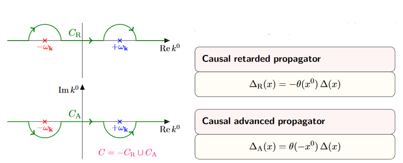
1. Apply Cauchy’s integral formula to find in the case $(x^0 – y^0)\gt 0$ the sum of the residues at these two poles times $2\pi i$, zero in the other case. (For the retarded propagator we get $- 2 \pi i$ times the residues, because now the contours encircling non-trivial poles go clockwise).
2. The result is now non-singular at $\epsilon = 0$ and therefore the limit $\epsilon \to 0$ is now computed by evaluating at $\epsilon = 0$.

This computation shows a) that the limiting distribution indeed exists, and b) that the support of $\Delta_+$ is in the future, and that of $\Delta_-$ is in the past.

Hence it only remains to see now that the support of $\Delta_\pm$ is inside the causal cone. But this follows from the previous argument, by using that the Klein-Gordon equation is invariant under Lorentz transformations: This implies that the support is in fact in the future of every spacelike slice through the origin in $\mathbb{R}^{p,1}$, hence in the closed future cone of the origin.

Corollary 9.53. (causal propagator is skew-symmetric)

Under reversal of arguments the advanced and retarded causal propagators from prop. 9.52 are related by

$$
\label{AdvancedAndRetardedPropagatorTurnIntoEachOtherUnderSwitchingArguments}
\Delta_{\pm}(y-x) = \Delta_\mp(x-y)
\,.
$$ (141)

It follows that the causal propagator (92) $\Delta := \Delta_+ – \Delta_-$ is skew-symmetric in its arguments:

$$
\Delta_S(x-y) = – \Delta_S(y-x)
\,.
$$

Proof. By prop. 9.52 we have with (132)

$$
\begin{aligned}
\Delta_\pm(y-x)
& =
\left\{
\array{
\frac{\pm i}{(2\pi)^{p}}
\int
\frac{1}{2\omega(\vec k)/c}
\left(
e^{-i \omega(\vec k)(x^0 – y^0)/c – i \vec k \cdot (\vec x -\vec y)}
–
e^{+i \omega(\vec k)(x^0 – y^0)/c – i \vec k \cdot (\vec x – \vec y) }
\right)
d^p \vec k
& \vert & \text{if} \, \mp (x^0 – y^0) \gt 0
\\
0 & \vert & \text{otherwise}
}
\right.
\\
& =
\left\{
\array{
\frac{\pm i}{(2\pi)^{p}}
\int
\frac{1}{2\omega(\vec k)/c}
\left(
e^{-i \omega(\vec k)(x^0 – y^0)/c + i \vec k \cdot (\vec x -\vec y)}
–
e^{+i \omega(\vec k)(x^0 – y^0)/c – i \vec k \cdot (\vec x – \vec y) }
\right)
d^p \vec k
& \vert & \text{if} \, \mp (x^0 – y^0) \gt 0
\\
0 & \vert & \text{otherwise}
}
\right.
\\
& =
\left\{
\array{
\frac{\mp i}{(2\pi)^{p}}
\int
\frac{1}{2\omega(\vec k)/c}
\left(
e^{+i \omega(\vec k)(x^0 – y^0)/c + i \vec k \cdot (\vec x -\vec y)}
–
e^{-i \omega(\vec k)(x^0 – y^0)/c – i \vec k \cdot (\vec x – \vec y) }
\right)
d^p \vec k
& \vert & \text{if} \, \mp (x^0 – y^0) \gt 0
\\
0 & \vert & \text{otherwise}
}
\right.
\\
& =
\Delta_\mp(x-y)
\end{aligned}
$$

Here in the second step we applied change of integration variables $\vec k \mapsto – \vec k$ (which introduces no sign because in addition to $d \vec k \mapsto – d \vec k$ the integration domain reverses orientation).

causal propagator

Proposition 9.54. (mode expansion of causal propagator for Klein-Gordon equation on Minkowski spacetime)

The causal propagator (92) for the Klein-Gordon equation for mass $m$ on Minkowski spacetime $\mathbb{R}^{p,1}$ (example 5.27) is given, in generalized function notation, by

$$
\label{CausalPropagatorModeExpansionForKleinGordonOnMinkowskiSpacetime}
\begin{aligned}
\Delta_S(x,y)
& =
\frac{+ i}{(2\pi)^{p}}
\int
\frac{1}{2\omega(\vec k)/c}
\left(
e^{i \omega(\vec k)(x^0 – y^0)/c + i \vec k \cdot (\vec x -\vec y)}
–
e^{-i \omega(\vec k)(x^0 – y^0)/c + i \vec k \cdot (\vec x – \vec y)}
\right)
d^p \vec k
\\
& =
\frac{-1}{(2\pi)^p}
\int
\frac{1}{\omega(\vec k)/c}
\sin\left( \omega(\vec k)(x^0 – y^0)/c \right)
e^{i \vec k \cdot (\vec x -\vec y)}
d^p \vec k
\,,
\end{aligned}
$$ (142)

where in the second line we used Euler’s formula $sin(\alpha)= \tfrac{1}{2i}\left( e^{i \alpha} – e^{-i \alpha} \right)$.

In particular this shows that the causal propagator is real, in that it is equal to its complex conjugate

$$
\label{CausalPropagatorForKleinGordonEquationOnMinkowskiSpacetimeIsReal}
\left(\Delta_S(x,y)\right)^\ast = \Delta_S(x,y)
\,.
$$ (143)

Proof. By definition and using the expression from prop. 9.52 for the advanced and retarded causal propagators we have

$$
\begin{aligned}
\Delta_S(x,y)
& :=
\Delta_+(x,y) – \Delta_-(x,y)
\\
& =
\left\{
\array{
\frac{+ i}{(2\pi)^{p}}
\int
\frac{1}{2\omega(\vec k)/c}
\left(
e^{i \omega(\vec k)(x^0 – y^0)/c + i \vec k \cdot (\vec x -\vec y)}
–
e^{-i \omega(\vec k)(x^0 – y^0)/c + i \vec k \cdot (\vec x – \vec y)}
\right)
d^p \vec k
& \vert & \text{if} \, + (x^0 – y^0) \gt 0
\\
\frac{(-1) (-1) i}{(2\pi)^{p}}
\int
\frac{1}{2\omega(\vec k)/c}
\left(
e^{i \omega(\vec k)(x^0 – y^0)/c + i \vec k \cdot (\vec x -\vec y)}
–
e^{-i \omega(\vec k)(x^0 – y^0)/c + i \vec k \cdot (\vec x – \vec y)}
\right)
d^p \vec k
& \vert & \text{if} \, – (x^0 – y^0) \gt 0
}
\right.
\\
& =
\frac{+ i}{(2\pi)^{p}}
\int
\frac{1}{2\omega(\vec k)/c}
\left(
e^{i \omega(\vec k)(x^0 – y^0)/c + i \vec k \cdot (\vec x -\vec y)}
–
e^{-i \omega(\vec k)(x^0 – y^0)/c + i \vec k \cdot (\vec x – \vec y)}
\right)
d^p \vec k
\\
& =
\frac{-1}{(2\pi)^p}
\int
\frac{1}{\omega(\vec k)/c}
\sin\left( \omega(\vec k)(x^0 – y^0)/c \right)
e^{i \vec k \cdot (\vec x -\vec y)}
d^p \vec k
\end{aligned}
$$

For the reality, notice from the last line that

$$
\begin{aligned}
\left(\Delta_S(x,y)\right)^\ast
& =
\frac{-1}{(2\pi)^p}
\int
\frac{1}{\omega(\vec k)/c}
\sin\left( \omega(\vec k)(x^0 – y^0)/c \right)
e^{-i \vec k \cdot (\vec x -\vec y)}
d^p \vec k
\\
& =
\frac{-1}{(2\pi)^p}
\int
\frac{1}{\omega(\vec k)/c}
\sin\left( \omega(\vec k)(x^0 – y^0)/c \right)
e^{+i \vec k \cdot (\vec x -\vec y)}
d^p \vec k
\\
& =
\Delta_S(x,y)
\,,
\end{aligned}
$$

where in the last step we used the change of integration variables $\vec k \mapsto – \vec k$ (which introduces no sign, since on top of $d \vec k \mapsto – d \vec k$ the orientation of the integration domain changes).

We consider a couple of equivalent expressions for the causal propagator which are useful for computations:

Proposition 9.55. (causal propagator for Klein-Gordon operator on Minkowski spacetime as a contour integral)

The causal propagator (prop. 7.24) for the Klein-Gordon equation at mass $m$ on Minkowski spacetime (example 5.27) has the following equivalent expression, as a generalized function, given as a contour integral along a Jordan curve $C(\vec k)$ going counter-clockwise around the two poles at $k_0 = \pm \omega(\vec k)/c$:

$$
\Delta_S(x,y)
\;=\;
(2\pi)^{-(p+1)}
\int
\underset{C(\vec k)}{\oint}
\frac{e^{i k_\mu (x-y)^\mu}}{ -k_\mu k^\mu – \left( \tfrac{m c}{\hbar} \right)^2g }
\,d k_0
\,d^{p} k
\,.
$$

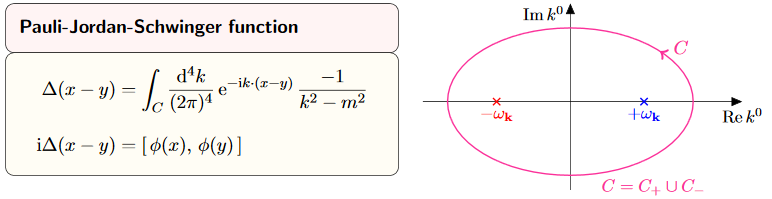
graphics grabbed from Kocic 16

Proof. By Cauchy’s integral formula we compute as follows:S

$$
\begin{aligned}
(2\pi)^{-(p+1)}
\int
\underset{C(\vec k)}{\oint}
\frac{e^{i k_\mu (x^\mu – y^\mu)}}{ -k_\mu k^\mu – \left( \tfrac{m c}{\hbar} \right)^2 }
\,d k_0
\,d^{p} k
& =
(2\pi)^{-(p+1)}
\int
\underset{C(\vec k)}{\oint}
\frac{
e^{i k_0 x^0} e^{ i \vec k \cdot (\vec x – \vec y)}
}{
k_0^2 – \omega(\vec k)^2/c^2
}
\,d k_0
\,d^p \vec k
\\
& =
(2\pi)^{-(p+1)}
\int
\underset{C(\vec k)}{\oint}
\frac{
e^{i k_0 (x^0 – y^0)} e^{i \vec k \cdot (\vec x – \vec y)}
}{
( k_0 + \omega(\vec k)/c )
( k_0 – \omega(\vec k)/c )
}
\,d k_0
\,d^p \vec k
\\
& =
(2\pi)^{-(p+1)}
2\pi i
\int
\left(
\frac{
e^{i \omega(\vec k) (x^0 – y^0)/c} e^{i \vec k \cdot (\vec x – \vec y)}
}
{
2 \omega(\vec k)/c
}
–
\frac{
e^{ – i \omega(\vec k) (x^0 – y^0)/c} e^{i \vec k \cdot (\vec x – \vec y)}
}{
2 \omega(\vec k)/c
}
\right)
\,d^p \vec k
\\
& =
i
(2\pi)^{-p}
\int
\frac{1}{\omega(\vec k)/c}
sin\left( \omega(\vec k)(x^0 – y^0)/c \right)
e^{i \vec k \cdot (\vec x – \vec y)}
\,d^p \vec k
\,.
\end{aligned}
$$

The last line is the expression for the causal propagator from prop. 9.54

Proposition 9.56. (causal propagator as Fourier transform of delta distribution on the Fourier transformed Klein-Gordon operator)

The causal propagator for the Klein-Gordon equation at mass $m$ on Minkowski spacetime has the following equivalent expression, as a generalized function:

$$
\Delta_S(x,y)
\;=\;
i (2\pi)^{-p} \int \delta\left( k_\mu k^\mu + \left( \tfrac{m c}{\hbar}\right)^2 \right) sgn( k_0 ) e^{ i k_\mu (x-y)^\mu } d^{p+1} k
\,,
$$

where the integrand is the product of the sign function of $k_0$ with the delta distribution of the Fourier transform of the Klein-Gordon operator and a plane wave factor.

Proof. By decomposing the integral over $k_0$ into its negative and its positive half, and applying the change of integration variables $k_0 = \pm\sqrt{h}$ we get

$$
\begin{aligned}
i (2\pi)^{-p} \int \delta\left( k_\mu k^\mu + \left( \tfrac{m c}{\hbar}\right)^2 \right) sgn( k_0 ) e^{ i k_\mu (x-y)^\mu } d^{p+1} k
& =
+ i (2\pi)^{-p} \int \int_0^\infty \delta\left( -k_0^2 + \vec k^2 + \left( \tfrac{m c}{\hbar}\right)^2 \right) e^{ i k_0 (x^0 – y^0) + i \vec k \cdot (\vec x – \vec y)} d k_0 \, d^p \vec k
\\
& \phantom{=}
– i (2\pi)^{-p} \int \int_{-\infty}^0 \delta\left( -k_0^2 + \vec k^2 + \left(\tfrac{m c}{\hbar}\right)^2 \right) e^{ i k_0 (x^0 – y^0)+ i \vec k \cdot (\vec x – \vec y) } d k_0 \, d^{p} \vec k
\\
& =
+i (2\pi)^{-p} \int \int_0^\infty \frac{1}{2 \sqrt{h}} \delta\left( -h + \omega(\vec k)^2/c^2 \right) e^{ + i \sqrt{h} (x^0 – y^0) + i \vec k \cdot \vec x } d h \, d^{p} \vec k
\\
& \phantom{=}
– i (2\pi)^{-p} \int \int_0^\infty \frac{1}{2 \sqrt{h}} \delta\left( – h + \omega(\vec k)^2/c^2 \right) e^{ – i \sqrt{h} (x^0 – y^0) + i \vec k \cdot \vec x } d h \, d^{p} \vec k
\\
& =
+i (2\pi)^{-p} \int \frac{1}{2 \omega(\vec k)/c} e^{ i \omega(\vec k) (x-y)^0/c + i \vec k \cdot \vec x} d^{p} \vec k
\\
& \phantom{=}
– i (2\pi)^{-p} \int \frac{1}{2 \omega(\vec k)/c} e^{ – i \omega(\vec k) (x-y)^0/c + i \vec k \cdot \vec x } d^{p} \vec k
\\
& = -(2 \pi)^{-p} \int \frac{1}{\omega(\vec k)/c}
sin\left( \omega(\vec k)(x-y)^0/c \right)
e^{i \vec k \cdot (\vec x – \vec y)}
\end{aligned}
$$

The last line is the expression for the causal propagator from prop. 9.54.

Wightman propagator

Prop. 9.56 exhibits the causal propagator of the Klein-Gordon operator on Minkowski spacetime as the difference of a contribution for positive temporal angular frequency $k_0 \propto \omega(\vec k)$ (hence positive energy $\hbar \omega(\vec k)$ and a contribution of negative temporal angular frequency.

The positive frequency contribution to the causal propagator is called the Wightman propagator (def. 9.57 below), also known as the the vacuum state 2-point function of the free real scalar field on Minkowski spacetime. Notice that the temporal component of the wave vector is proportional to the negative angular frequency

$$
k_0 = -\omega/c
$$

(see at plane wave), therefore the appearance of the step function $\Theta(-k_0)$ in (144) below:

Definition 9.57. (Wightman propagator or vacuum state 2-point function for Klein-Gordon operator on Minkowski spacetime)

The Wightman propagator for the Klein-Gordon operator at mass $m$ on Minkowski spacetime (example 5.27) is the tempered distribution in two variables $\Delta_H \in \mathcal{S}'(\mathbb{R}^{p,1})$ which as a generalized function is given by the expression

$$
\label{HadamardPropagatorForKleinGordonOperatorOnMinkowskiSpacetime}
\begin{aligned}
\Delta_H(x,y)
& :=
\frac{1}{(2\pi)^p} \int \delta\left( k_\mu k^\mu + m^2 \right) \Theta( -k_0 ) e^{i k_\mu (x^\mu-y^\mu) } \, d^{p+1} k
\\
& =
\frac{1}{(2\pi)^p}
\int \frac{1}{2 \omega(\vec k)/c}
e^{-i \omega(\vec k)(x^0 – y^0)/c + i \vec k \cdot (\vec x – \vec y) }
\, d^p \vec k
\,,
\end{aligned}
$$ (144)

Here in the first line we have in the integrand the delta distribution of the Fourier transform of the Klein-Gordon operator times a plane wave and times the step function $\Theta$ of the temporal component of the wave vector. In the second line we used the change of integration variables $k_0 = \sqrt{h}$, then the definition of the delta distribution and the fact that $\omega(\vec k)$ is by definition the non-negative solution to the Klein-Gordon dispersion relation.

(e.g. Khavkine-Moretti 14, equation (38) and section 3.4)

Proposition 9.58. (Wightman propagator on Minkowski spacetime is distributional solution to Klein-Gordon equation)

The Wightman propagator $\Delta_H$ (def. 9.57) is a distributional solution (def. 7.16) to the Klein-Gordon equation

$$
(\Box_x – m^2)\Delta_H(x,y) = 0
\,.
$$

Proof. By definition 9.57 the Wightman propagator is the Fourier transform of distributions of the product of distributions

$$
\delta(k_\mu k^\mu + m^2) \Theta(-k_0)
\,,
$$

where in turn the argument of the delta distribution is just $-1$ times the Fourier transform of the [Klein-Gordon operator]] itself (prop. 9.8). This is clearly a solution to the equation

$$
(-k_\mu k^\mu – m^2) \, \delta(k_\mu k^\mu + m^2) \Theta(-k_0)
\;=\;
0
\,.
$$

Under Fourier inversion (prop. 9.7), this is the equation $(\Box_x – m^2)\Delta_H(x,y) = 0$, as in the proof of prop. 9.52.

Proposition 9.59. (contour integral representation of the Wightman propagator for the Klein-Gordon operator on Minkowski spacetime)

The Wightman propagator from def. 9.57 is equivalently given by the contour integral

$$
\label{StandardHadamardPropagatorOnMinkowskiSpacetimeInTermsOfContourIntegral}
\Delta_H(x,y)
\;=\;
-i(2\pi)^{-(p+1)}
\int
\underset{C_+(\vec k)}{\oint}
\frac{e^{-i k_\mu (x-y)^\mu}}{ -k_\mu k^\mu – \left( \tfrac{m c}{\hbar} \right)^2 }
d k_0
d^{p} k
\,,
$$ (145)

where the Jordan curve $C_+(\vec k) \subset \mathbb{C}$ runs counter-clockwise, enclosing the point $+ \omega(\vec k)/c \in \mathbb{R} \subset \mathbb{C}$, but not enclosing the point $- \omega(\vec k)/c \in \mathbb{R} \subset \mathbb{C}$.

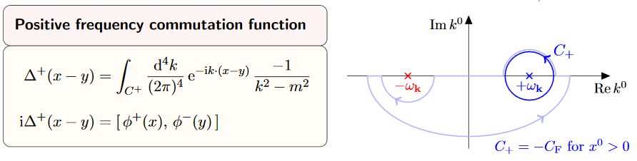
graphics grabbed from Kocic 16

Proof. We compute as follows:

$$
\begin{aligned}
-i(2\pi)^{-(p+1)}
\int
\underset{C_+(\vec k)}{\oint}
\frac{e^{ – i k_\mu (x-y)^\mu}}{ -k_\mu k^\mu – \left( \tfrac{m c}{\hbar} \right)^2 }
d k_0
d^{p} k
& =
-i(2\pi)^{-(p+1)}
\int
\oint_{C_+(\vec k)}
\frac{
e^{ -i k_0 x^0} e^{i \vec k \cdot (\vec x – \vec y)}
}{
k_0^2 – \omega(\vec k)^2/c^2
}
d k_0
d^p \vec k
\\
& =
-i(2\pi)^{-(p+1)}
\int
\underset{C_+(\vec k)}{\oint}
\frac{
e^{ – i k_0 (x^0-y^0)} e^{i \vec k \cdot (\vec x – \vec y)}
}{
( k_0 – \omega_\epsilon(\vec k) )
( k_0 + \omega_\epsilon(\vec k) )
}
d k_0
d^p \vec k
\\
& =
(2\pi)^{-p}
\int
\frac{1}{2 \omega(\vec k)}
e^{-i \omega(\vec k) (x^0-y^0)/c} e^{i \vec k \cdot (\vec x – \vec y)}
d^p \vec k
\,.
\end{aligned}
$$

The last step is the application of Cauchy’s integral formula, which says that the contour integral picks up the residue of the pole of the integrand at $+ \omega(\vec k)/c \in \mathbb{R} \subset \mathbb{C}$. The last line is $\Delta_H(x,y)$, by definition 9.57.

Proposition 9.60. (skew-symmetric part of Wightman propagator is the causal propagator)

The Wightman propagator for the Klein-Gordon equation on Minkowski spacetime (def. 9.57) is of the form

$$
\label{DeompositionOfHadamardPropagatorOnMinkowkski}
\begin{aligned}
\Delta_H
& =
\tfrac{i}{2} \Delta_S
+
H
\\
& =
\tfrac{i}{2}
\left(
\Delta_+ – \Delta_-
\right)
+
H
\end{aligned}
\,,
$$ (146)

where

1. $\Delta_S$ is the causal propagator (prop. 9.52), which is real (143) and skew-symmetric (prop. 9.53)$$
   (\Delta_S(x,y))^\ast = \Delta_S(x,y)
   \phantom{AA}
   \,,
   \phantom{AA}
   \Delta_S(y,x) = – \Delta_S(x,y)
   $$
2. $H$ is real and symmetric
   

   $$
   \label{RealAndSymmetricH}
   (H(x,y))^\ast = H(x,y)
   \phantom{AA}
   \,,
   \phantom{AA}
   H(y,x) = H(x,y)
   $$ (147)

Proof. By applying Euler’s formula to (144) we obtain

$$
\label{SymmetricPartOfHadamardPropagatorForKleinGordonOnMinkowskiSpacetime}
\begin{aligned}
\Delta_H(x,y)
& =
\frac{1}{(2\pi)^p}
\int \frac{1}{2 \omega(\vec k)/c}
e^{-i \omega(\vec k)(x^0 – y^0)/c + i \vec k \cdot (\vec x – \vec y) }
\, d^p \vec k
\\
& =
\tfrac{i}{2}
\underset{= \Delta_S(x,y)}{
\underbrace{
\frac{-1}{(2\pi)^p}
\int
\frac{1}{\omega(\vec k)/c}
\sin\left( \omega(\vec k)(x^0 – y^0)/c \right)
e^{i \vec k \cdot (\vec x – \vec y) }
\, d^p \vec k
}}
\;+\;
\underset{
:= H(x,y)
}{
\underbrace{
\frac{1}{(2\pi)^p}
\int \frac{1}{2 \omega(\vec k)/c}
\cos\left( \omega(\vec k)(x^0 – y^0)/c \right)
e^{i \vec k \cdot (\vec x – \vec y) }
\, d^p \vec k
}}
\end{aligned}
$$ (148)

On the left this identifies the causal propagator by (142), prop. 9.54.

The second summand changes, both under complex conjugation as well as under $(x-y) \mapsto (y-x)$, via change of integration variables $\vec k \mapsto – \vec k$ (because the cosine is an even function). This does not change the integral, and hence $H$ is symmetric.

Feynman propagator

We have seen that the positive frequency component of the causal propagator $\Delta_S$ for the Klein-Gordon equation on Minkowski spacetime (prop. 9.52) is the Wightman propagator $\Delta_H$ (def. 9.57) given, according to prop. 9.60, by (146)

$$
\begin{aligned}
\Delta_H
& =
\tfrac{i}{2} \Delta_S
+
H
\\
& =
\tfrac{i}{2}
\left(
\Delta_+ – \Delta_-
\right)
+
H
\end{aligned}
\,,
$$

There is an evident variant of this combination, which will be of interest:

Definition 9.61. (Feynman propagator for Klein-Gordon equation on Minkowski spacetime)

The Feynman propagator for the Klein-Gordon equation on Minkowski spacetime (example 5.27) is the linear combination

$$
\Delta_F
:=
\tfrac{i}{2}
\left(
\Delta_+ + \Delta_-
\right)
+
H
$$

where the first term is proportional to the sum of the advanced and retarded propagators (prop. 9.52) and the second is the symmetric part of the Wightman propagator according to prop. 9.60.

Similarly, the anti-Feynman propagator is

$$
\Delta_{\overline{F}}
:=
\tfrac{i}{2}
\left(
\Delta_+ + \Delta_-
\right)
–
H
\,.
$$

It follows immediately that:

Proposition 9.62. (Feynman propagator is symmetric)

The Feynman propagator $\Delta_F$ and anti-Feynman propagator $\Delta_{\overline{F}}$ (def. 9.61) are symmetric:

$$
\Delta_F(x,y) = \Delta_F(y,x)
\,.
$$

Proof. By equation (141) in cor. 9.53 we have that $\Delta_+ + \Delta_-$ is symmetric, and equation (147) in prop. 9.60 says that $H$ is symmetric.

Proposition 9.63. (mode expansion for Feynman propagator of Klein-Gordon equation on Minkowski spacetime)

The Feynman propagator (def. 9.61) for the Klein-Gordon equation on Minkowski spacetime is given by the following equivalent expressions

$$
\begin{aligned}
\Delta_F(x,y)
& =
\left\{
\array{
\frac{1}{(2\pi)^p}
\int
\frac{1}{\omega(\vec k)c}
e^{-i\omega(\vec k)(x^0 – y^0)/c} e^{i \vec k \cdot (\vec x – \vec y)}
\, d^p \vec k
&\vert&
(x^0 – y^0) \gt 0
\\
\frac{1}{(2\pi)^p}
\int
\frac{1}{2\omega(\vec k)c}
e^{+i\omega(\vec k)(x^0 – y^0)/c} e^{i \vec k \cdot (\vec x – \vec y)}
\, d^p \vec k
&\vert&
(x^0 – y^0) \lt 0
}
\right.
\\
& =
\left\{
\array{
\Delta_H(x,y) &\vert& (x^0 – y^0) \gt 0
\\
\Delta_H(y,x) &\vert& (x^0 – y^0) \lt 0
}
\right.
\end{aligned}
$$

Similarly the anti-Feynman propagator is equivalently given by

$$
\begin{aligned}
\Delta_{\overline{F}}(x,y)
& =
\left\{
\array{
\frac{-}{(2\pi)^p}
\int
\frac{1}{\omega(\vec k)c}
e^{+i\omega(\vec k)(x^0 – y^0)/c} e^{i \vec k \cdot (\vec x – \vec y)}
\, d^p \vec k
&\vert&
(x^0 – y^0) \gt 0
\\
\frac{-}{(2\pi)^p}
\int
\frac{1}{2\omega(\vec k)c}
e^{-i\omega(\vec k)(x^0 – y^0)/c} e^{i \vec k \cdot (\vec x – \vec y)}
\, d^p \vec k
&\vert&
(x^0 – y^0) \lt 0
}
\right.
\\
& =
\left\{
\array{
-\Delta_H(y,x) &\vert& (x^0 – y^0) \gt 0
\\
-\Delta_H(x,y) &\vert& (x^0 – y^0) \lt 0
}
\right.
\end{aligned}
$$

Proof. By the mode expansion of $\Delta_{\pm}$ from (132) and the mode expansion of $H$ from (148) we have

$$
\begin{aligned}
\Delta_F(x,y)
& =
\left\{
\array{
\underset{
= \tfrac{i}{2} \Delta_+(x,y) + 0 \;\text{for}\; (x^0 – y^0) \gt 0
}{
\underbrace{
\frac{- i}{(2\pi)^{p}}
\int
\frac{1}{2 \omega(\vec k)/c}
\sin\left( \omega(\vec k)(x^0 – y^0)/c \right)
e^{i \vec k \cdot (\vec x – \vec y) }
\, d^p \vec k
}
}
+
\underset{
= H(x,y)
}{
\underbrace{
\frac{1}{(2\pi)^p}
\int \frac{1}{2 \omega(\vec k)/c}
\cos\left( \omega(\vec k)(x^0 – y^0)/c \right)
e^{i \vec k \cdot (\vec x – \vec y) }
\, d^p \vec k
}
}
&\vert&
(x^0 – y^0) \gt 0
\\
\underset{
= 0 + \tfrac{i}{2}\Delta_-(x,y) \;\text{for}\; (x^0 – y^0) \lt 0
}{
\underbrace{
\frac{+ i}{(2\pi)^{p}}
\int
\frac{1}{2 \omega(\vec k)/c}
\sin\left( \omega(\vec k)(x^0 – y^0)/c \right)
e^{i \vec k \cdot (\vec x – \vec y) }
\, d^p \vec k
}
}
+
\underset{ = H(x,y) }{
\underbrace{
\frac{1}{(2\pi)^p}
\int \frac{1}{2 \omega(\vec k)/c}
\cos\left( \omega(\vec k)(x^0 – y^0)/c \right)
e^{i \vec k \cdot (\vec x – \vec y) }
\, d^p \vec k
}
}
&\vert&
(x^0 – y^0) \lt 0
}
\right.
\\
& =
\left\{
\array{
\frac{1}{(2\pi)^p}
\int
\frac{1}{2\omega(\vec k)c}
e^{-i\omega(\vec k)(x^0 – y^0)/c} e^{i \vec k \cdot (\vec x – \vec y)}
\, d^p \vec k
&\vert&
(x^0 – y^0) \gt 0
\\
\frac{1}{(2\pi)^p}
\int
\frac{1}{2\omega(\vec k)c}
e^{+i\omega(\vec k)(x^0 – y^0)/c} e^{i \vec k \cdot (\vec x – \vec y)}
\, d^p \vec k
&\vert&
(x^0 – y^0) \lt 0
}
\right.
\\
& =
\left\{
\array{
\Delta_H(x,y) &\vert& (x^0 – y^0) \gt 0
\\
\Delta_H(y,x) &\vert& (x^0 – y^0) \lt 0
}
\right.
\end{aligned}
$$

where in the second line we used Euler’s formula. The last line follows by comparison with (144) and using that the integral over $\vec k$ is invariant under $\vec k \mapsto – \vec k$.

The computation for $\Delta_{\overline{F}}$ is the same, only now with a minus sign in front of the cosine:

$$
\begin{aligned}
\Delta_{\overline{F}}(x,y)
& =
\left\{
\array{
\underset{
= \tfrac{i}{2} \Delta_+(x,y) + 0 \;\text{for}\; (x^0 – y^0) \gt 0
}{
\underbrace{
\frac{- i}{(2\pi)^{p}}
\int
\frac{1}{2 \omega(\vec k)/c}
\sin\left( \omega(\vec k)(x^0 – y^0)/c \right)
e^{i \vec k \cdot (\vec x – \vec y) }
\, d^p \vec k
}
}
–
\underset{
= H(x,y)
}{
\underbrace{
\frac{1}{(2\pi)^p}
\int \frac{1}{2 \omega(\vec k)/c}
\cos\left( \omega(\vec k)(x^0 – y^0)/c \right)
e^{i \vec k \cdot (\vec x – \vec y) }
\, d^p \vec k
}
}
&\vert&
(x^0 – y^0) \gt 0
\\
\underset{
= 0 + \tfrac{i}{2}\Delta_-(x,y) \;\text{for}\; (x^0 – y^0) \lt 0
}{
\underbrace{
\frac{+ i}{(2\pi)^{p}}
\int
\frac{1}{2 \omega(\vec k)/c}
\sin\left( \omega(\vec k)(x^0 – y^0)/c \right)
e^{i \vec k \cdot (\vec x – \vec y) }
\, d^p \vec k
}
}
–
\underset{ = H(x,y) }{
\underbrace{
\frac{1}{(2\pi)^p}
\int \frac{1}{2 \omega(\vec k)/c}
\cos\left( \omega(\vec k)(x^0 – y^0)/c \right)
e^{i \vec k \cdot (\vec x – \vec y) }
\, d^p \vec k
}
}
&\vert&
(x^0 – y^0) \lt 0
}
\right.
\\
& =
\left\{
\array{
\frac{-1}{(2\pi)^p}
\int
\frac{1}{2\omega(\vec k)c}
e^{+i\omega(\vec k)(x^0 – y^0)/c} e^{i \vec k \cdot (\vec x – \vec y)}
\, d^p \vec k
&\vert&
(x^0 – y^0) \gt 0
\\
\frac{-1}{(2\pi)^p}
\int
\frac{1}{2\omega(\vec k)c}
e^{-1i\omega(\vec k)(x^0 – y^0)/c} e^{i \vec k \cdot (\vec x – \vec y)}
\, d^p \vec k
&\vert&
(x^0 – y^0) \lt 0
}
\right.
\\
& =
\left\{
\array{
– \Delta_H(y,x) &\vert& (x^0 – y^0) \gt 0
\\
– \Delta_H(x,y) &\vert& (x^0 – y^0) \lt 0
}
\right.
\end{aligned}
$$

As before for the causal propagator, there are equivalent reformulations of the Feynman propagator which are useful for computations:

Proposition 9.64. (Feynman propagator as a Cauchy principal value)

The Feynman propagator and anti-Feynman propagator (def. 9.61) for the Klein-Gordon equation on Minkowski spacetime is equivalently given by the following expressions, respectively:

$$
\begin{aligned}
\left.
\array{
\Delta_F(x,y)
\\
\Delta_{\overline{F}}(x,y)
}
\right\}
& =
\underset{ {\epsilon \in (0,\infty)} \atop {\epsilon \to 0} }{\lim}
\frac{+i}{(2\pi)^{p+1}}
\int
\int_{-\infty}^\infty
\frac{
e^{i k_\mu (x^\mu – y^\mu)}
}{
– k_\mu k^\mu – \left( \tfrac{m c}{\hbar} \right)^2 \pm i \epsilon
}
\, d k_0 \, d^p \vec k
\end{aligned}
$$

where we have a limit of distributions as for the Cauchy principal value (this prop).

Proof. We compute as follows:

$$
\begin{aligned}
\underset{ {\epsilon \in (0,\infty)} \atop {\epsilon \to 0} }{\lim}
\frac{i}{(2\pi)^{p+1}}
\int
\int_{-\infty}^\infty
\frac{
e^{i k_\mu (x^\mu – y^\mu)}
}{
– k_\mu k^\mu – \left( \tfrac{m c}{\hbar} \right)^2 \pm i \epsilon
}
\, d k_0 \, d^p \vec k
& =
\underset{ {\epsilon \in (0,\infty)} \atop {\epsilon \to 0} }{\lim}
\frac{i}{(2\pi)^{p+1}}
\int
\int_{-\infty}^\infty
\frac{
e^{i k_\mu (x^\mu – y^\mu)}
}{
(k_0)^2
–
\underset{
:= \omega_{\pm\epsilon}(\vec k)^2/c^2
}{\underbrace{ \left( \omega(\vec k)^2/c^2 \pm i \epsilon \right) }}
}
\, d k_0 \, d^p \vec k
\\
& =
\underset{ {\epsilon \in (0,\infty)} \atop {\epsilon \to 0} }{\lim}
\frac{i}{(2\pi)^{p+1}}
\int
\int_{-\infty}^\infty
\frac{
e^{i k_\mu (x^\mu – y^\mu)}
}{
\left(
k_0 – \omega_{\pm \epsilon}(\vec k)/c
\right)
\left(
k_0 + \omega_{\pm \epsilon}(\vec k)/c
\right)
}
\, d k_0 \, d^p \vec k
\\
& =
\left\{
\array{
\frac{\mp 1}{(2\pi)^p}
\int
\frac{1}{2\omega(\vec k)c}
e^{\pm i\omega(\vec k)(x^0 – y^0)/c} e^{i \vec k \cdot (\vec x – \vec y)}
\, d^p \vec k
&\vert&
(x^0 – y^0) \gt 0
\\
\frac{\mp 1}{(2\pi)^p}
\int
\frac{1}{2\omega(\vec k)c}
e^{\mp i\omega(\vec k)(x^0 – y^0)/c} e^{i \vec k \cdot (\vec x – \vec y)}
\, d^p \vec k
&\vert&
(x^0 – y^0) \lt 0
}
\right.
\\
& =
\left\{
\array{
\Delta_F(x,y)
\\
\Delta_{\overline{F}}(x,y)
}
\right.
\end{aligned}
$$

Here

1. In the first step we introduced the complex square root $\omega_{\pm \epsilon}(\vec k)$. For this to be compatible with the choice of non-negative square root for $\epsilon = 0$ in (131) we need to choose that complex square root whose complex phase is one half that of $\omega(\vec k)^2 – i \epsilon$ (instead of that plus π). This means that $\omega_{+ \epsilon}(\vec k)$ is in the upper half plane and $\omega_-(\vec k)$ is in the lower half plane.
2. In the third step we observe that
   1. for $(x^0 – y^0) \gt 0$ the integrand decays for positive imaginary part and hence the integration over $k_0$ may be deformed to a contour which encircles the pole in the upper half plane;
   2. for $(x^0 – y^0) \lt 0$ the integrand decays for negative imaginary part and hence the integration over $k_0$ may be deformed to a contour which encircles the pole in the lower half plane

   and then apply Cauchy’s integral formula which picks out $2\pi i$ times the residue a these poles.

   

   Notice that when completing to a contour in the lower half plane we pick up a minus signs from the fact that now the contour runs clockwise.

3. In the fourth step we used prop. 9.63.

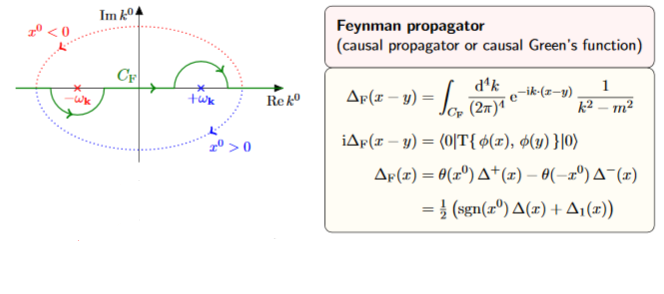
It follows that:

Corollay 9.65. (Feynman propagator is Green function)

The Feynman propagator $\Delta_F$ for the Klein-Gordon equation on Minkowski spacetime (def. 9.61) is proportional to a Green function for the Klein-Gordon equation in that

$$
\left( \Box_x – \left( \tfrac{m c}{\hbar}\right)^2 \right) \Delta_{F}(x,y)
=
(+i) \delta(x-y)
\,.
$$

Proof. Equation link in prop. 9.64 says that the Feynman propagator is the inverse Fourier transform of distributions of

$$
\widehat{\Delta_F}(k)
\;=\;
(+i)
\underset{ {\epsilon \in (0,\infty)} \atop {\epsilon \to 0} }{\lim}
\frac{
1
}{
– k_\mu k^\mu – \left( \tfrac{m c}{\hbar} \right)^2 \pm i \epsilon
}
$$

This implies the statement as in the proof of prop. 9.52, via the analogue of equation (138).

singular support and wave front sets

We now discuss the singular support (def. 9.24) and the wave front sets (def. 9.28) of the various propagators for the Klein-Gordon equation on Minkowski spacetime.

Proposition 9.66. (singular support of the causal propagator of the Klein-Gordon equation on Minkowski spacetime is the light cone)

The singular support of the causal propagator $\Delta_S$ for the Klein-Gordon equation on Minkowski spacetime, regarded via translation invariance as a generalized function in a single variable (133) is the light cone of the origin:

$$
supp_{sing}(\Delta_S)
\;=\;
\left\{
x \in \mathbb{R}^{p,1}
\,\vert\,
{\vert x\vert}^2_\eta = 0
\right\}
\,.
$$

Proof. By prop. 9.56 the causal propagator is equivalently the Fourier transform of distributions of the delta distribution of the mass shell times the sign function of the angular frequency; and by the basic properties of the Fourier transform (prop. 9.8) this is the convolution of distributions of the separate Fourier transforms:

$$
\begin{aligned}
\Delta_S(x)
& \propto
\widehat{
\delta\left( \eta^{-1}(k,k) + \left( \tfrac{m c}{\hbar}\right)^2 \right) sgn( k_0 )
}
\\
&\propto
\widehat{\delta\left( \eta^{-1}(k,k) + \left( \tfrac{m c}{\hbar}\right)^2 \right)}
\star
\widehat{sgn( k_0 )}
\end{aligned}
$$

By prop. 9.51, the singular support of the first convolution factor is the light cone.

The second factor is

$$
\begin{aligned}
\widehat{sgn(k_0)}
& \propto
\left(2\widehat{\Theta(k_0)} – \widehat{1}\right) \delta(\vec k)
\\
& \propto
\left(2\tfrac{1}{i x^0 + 0^+} – \delta(x^0)\right) \delta(\vec k)
\end{aligned}
$$

(by example 9.18 and example 9.49) and hence the wave front set (def. 9.28) of the second factor is

$$
WF\left(\widehat{sgn(k_0)}\right) = \{(0,k) \;\vert\; k \in S(\mathbb{R}^{p+1})\}
$$

(by example 9.31 and example 9.44).

With this the statement follows, via a partition of unity, from this prop..

For illustration we now make this general argument more explicit in the special case of spacetime dimension

$$
p + 1 = 3 + 1
$$

by computing an explicit form for the causal propagator in terms of the delta distribution, the Heaviside distribution and smooth Bessel functions.

We follow (Scharf 95 (2.3.18)).

Consider the formula for the causal propagator in terms of the mode expansion (142). Since the integrand here depends on the wave vector $\vec k$ only via its norm ${\vert \vec k\vert}$ and the angle $\theta$ it makes with the given spacetime vector via

$$
\vec k \cdot (\vec x – \vec y)
\;=\;
{\vert \vec k\vert} \, {\vert \vec x\vert} \, \cos(\theta)
$$

we may express the integration in terms of polar coordinates as follws:

$$
\begin{aligned}
\Delta_S(x – y)
& =
\frac{-1}{(2\pi)^p}
\int \frac{1}{2 \omega(\vec k)/c}
\sin\left( \omega(\vec k)(x^0 – y^0)/c \right)
e^{i \vec k \cdot (\vec x – \vec y)}
\, d^p \vec k
\\
& =
\frac{- vol_{S^{p-2}}}{(2\pi)^p}
\underset{{\vert \vec k\vert} \in \mathbb{R}_{\geq 0}}{\int}
\underset{ \theta \in [0,\pi] }{\int}
\frac{ 1 }{ \omega(\vec k)/c }
\sin\left( \omega(\vec k) (x^0 – y^0) /c \right)
e^{ i {\vert \vec k\vert} {\vert \vec x – \vec y\vert} \cos(\theta) }
{\vert \vec k\vert} ({\vert \vec k\vert} \sin(\theta))^{p-2}
\,
d \theta
\wedge
d {\vert \vec k\vert}
\end{aligned}
$$

In the special case of spacetime dimension $p + 1 = 3 + 1$ this becomes

$$
\label{StepsInComputingCausalPropagatorIn3plus1Dimension}
\begin{aligned}
\Delta_S(x – y)
& =
\frac{- 2\pi}{(2\pi)^{3}}
\underset{{\vert \vec k\vert} \in \mathbb{R}_{\geq 0}}{\int}
\frac{ {\vert \vec k \vert}^2 }{ \omega(\vec k)/c }
\sin\left( \omega(\vec k) (x^0 – y^0) /c \right)
\underset{
=
\tfrac{1}{i {\vert \vec k\vert}\, {\vert \vec x – \vec y\vert} }
\left(
e^{i {\vert \vec k\vert}\, {\vert \vec x – \vec y\vert}}
–
e^{-i {\vert \vec k\vert}\, {\vert \vec x – \vec y\vert}}
\right)
}{
\underbrace{
\underset{ \cos(\theta) \in [-1,1] }{\int}
e^{ i {\vert \vec k\vert} {\vert \vec x – \vec y\vert} \cos(\theta) }
d \cos(\theta)
}
}
\wedge
d {\vert \vec k \vert}
\\
& =
\frac{- 2}{(2\pi)^{2} {\vert \vec x – \vec y\vert}}
\underset{{\vert \vec k\vert} \in \mathbb{R}_{\geq 0}}{\int}
\frac{ {\vert \vec k \vert} }{ \omega(\vec k)/c }
\sin\left( \omega(\vec k) (x^0 – y^0) /c \right)
\sin\left( {\vert \vec k\vert}\, {\vert \vec x – \vec y\vert} \right)
\, d {\vert \vec k\vert}
\\
& =
\frac{- 2}{(2\pi)^{2} {\vert \vec x – \vec y\vert}}
\frac{d}{d {\vert \vec x – \vec y \vert } }
\underset{{\vert \vec k\vert} \in \mathbb{R}_{\geq 0}}{\int}
\frac{ 1 }{ \omega(\vec k)/c }
\sin\left( \omega(\vec k) (x^0 – y^0) /c \right)
\cos\left( {\vert \vec k\vert}\, {\vert \vec x – \vec y\vert} \right)
\, d {\vert \vec k\vert}
\\
& =
\frac{- 1}{(2\pi)^{2} {\vert \vec x – \vec y\vert}}
\frac{d}{d {\vert \vec x – \vec y \vert } }
\underset{ \kappa \in \mathbb{R} }{\int}
\frac{ 1 }{ \omega(\kappa)/c }
\sin\left( \omega(\kappa) (x^0 – y^0) /c \right)
\cos\left( \kappa\, {\vert \vec x – \vec y\vert} \right)
\, d \kappa
\\
& =
\frac{- 1}{2(2\pi)^{2} {\vert \vec x – \vec y\vert}}
\frac{d}{d {\vert \vec x – \vec y} \vert }
\left(
\underset{:= I_+}{
\underbrace{
\underset{ \kappa \in \mathbb{R} }{\int}
\frac{ 1 }{ \omega(\kappa)/c }
\sin\left(
\omega(\kappa) (x^0 – y^0) /c
+
\kappa\, {\vert \vec x – \vec y\vert}
\right)
d\kappa
}
}
+
\underset{ := I_- }{
\underbrace{
\underset{ \kappa \in \mathbb{R} }{\int}
\frac{ 1 }{ \omega(\kappa)/c }
\sin\left(
\omega(\kappa) (x^0 – y^0) /c
–
\kappa\, {\vert \vec x – \vec y\vert}
\right)
\,
d \kappa
}
}
\right)
\,.
\end{aligned}
$$ (149)

Here in the second but last step we renamed $\kappa := {\vert \vec k\vert}$ and doubled the integration domain for convenience, and in the last step we used the trigonometric identity $\sin(\alpha) \cos(\beta)\;=\; \tfrac{1}{2} \left( \sin(\alpha + \beta) + \sin(\alpha – \beta) \right)$.

In order to further evaluate this, we parameterize the remaining components $(\omega/c, \kappa)$ of the wave vector by the dual rapidity $z$, via

$$
\left(\cosh(z)\right)^2 – \left( \sinh(z)\right)^2 = 1
$$

as

$$
\omega(\kappa)/c
\;=\;
\left(
\tfrac{m c}{\hbar}
\right)
\cosh(z)
\phantom{AA}
\,,
\phantom{AA}
\kappa
\;=\;
\left(
\tfrac{m c}{\hbar}
\right)
\sinh(z)
\,,
$$

which makes use of the fact that $\omega(\kappa)$ is non-negative, by construction. This change of integration variables makes the integrals under the braces above become

$$
\label{TheTwoSpecialFunctionIntegralsInTheComputationOfTheCausalPropagatorIn3Plus1DOnMinkowski}
I_\pm
\;=\;
\int_{-\infty}^\infty
\sin\left(
\tfrac{m c}{\hbar}
\left(
(x^0 – y^0) \cosh(z)
\pm
{\vert \vec x – \vec y\vert}
\sinh(z)
\right)
\right)
\, d z
\,.
$$ (150)

Next we similarly parameterize the vector $x-y$ by its rapidity $\tau$. That parameterization depends on whether $x-y$ is spacelike or not, and if not, whether it is future or past directed.

First, if $x-y$ is spacelike in that ${\vert x-y\vert}^2_\eta \gt 0$ then we may parameterize as

$$
(x^0 – y^0)
=
\sqrt{{\vert x-y\vert}^2_\eta} \sinh(\tau)
\phantom{AA}
\,,
\phantom{AA}
{\vert \vec x – \vec y\vert}
=
\sqrt{ {\vert x-y\vert}^2_\eta} \cosh(\tau)
$$

which yields

$$
\begin{aligned}
I_{\pm}
& =
\int_{-\infty}^\infty
\sin\left(
\tfrac{m c}{\hbar}
\sqrt{ {\vert x-y\vert}^2_\eta }
\left(
\sinh(\tau) \cosh(z)
\pm
\cosh(\tau)
\sinh(z)
\right)
\right)
\, d z
\\
& =
\int_{-\infty}^\infty
\sin\left(
\tfrac{m c}{\hbar}
\sqrt{ {\vert x-y\vert}^2_\eta}
\left(
\sinh\left( \tau \pm z\right)
\right)
\right)
\, d z
\\
& =
\int_{-\infty}^\infty
\sin\left(
\tfrac{m c}{\hbar}
\sqrt{ {\vert x-y\vert}^2_\eta }
\left(
\sinh\left( z \right)
\right)
\right)
\, d z
\\
& = 0
\,,
\end{aligned}
$$

where in the last line we observe that the integrand is a skew-symmetric function of $z$.

Second, if $x-y$ is timelike with $(x^0 – y^0) \gt 0$ then we may parameterize as

$$
(x^0 – y^0)
=
\sqrt{ -{\vert x-y\vert}^2_\eta} \cosh(\tau)
\phantom{AA}
\,,
\phantom{AA}
{\vert \vec x – \vec y\vert}
=
\sqrt{ -{\vert x – y\vert}^2_\eta }
\sinh(\tau)
$$

which yields

$$
\label{IdentifyingTheBesselFunctionInComputationOfCausalPropagatorIn3Plus1DOnMinkowski}
\begin{aligned}
I_\pm
& =
\int_{-\infty}^\infty
\sin\left(
\tfrac{m c}{\hbar}
\left(
(x^0 – y^0) \cosh(z)
\pm
{\vert \vec x – \vec y\vert}
\sinh(z)
\right)
\right)
\, d z
\\
& =
\int_{-\infty}^\infty
\sin\left(
\sqrt{ – {\vert x-y\vert}^2_\eta }
\tfrac{m c}{\hbar}
\left(
\cosh(\tau)\cosh(z)
\pm
\cosh(\tau)
\sinh(z)
\right)
\right)
\, d z
\\
& =
\int_{-\infty}^\infty
\sin\left(
\sqrt{ – {\vert x-y\vert}^2_\eta }
\tfrac{m c}{\hbar}
\left(
\cosh(z \pm \tau)
\right)
\right)
\, d z
\\
& =
\pi J_0\left( \sqrt{ – {\vert x-y\vert}^2_\eta} \tfrac{m c}{\hbar} \right)
\end{aligned}
\,.
$$ (151)

Here in the last line we identified the integral representation of the Bessel function $J_0$ of order 0 (see here). The important point here is that this is a smooth function.

Similarly, if $x-y$ is timelike with $(x^0 – y^0) \lt 0$ then the same argument yields

$$
I_\pm = – \pi J_0\left( \sqrt{ – {\vert x-y\vert}^2_\eta} \tfrac{m c}{\hbar} \right)
$$

In conclusion, the general form of $I_\pm$ is

$$
I_\pm
=
\pi
sgn(x^0 – y^0)
\Theta\left( -{\vert x-y\vert}^2_\eta \right)
J_0\left( \sqrt{ – {\vert x-y\vert}^2_\eta } \tfrac{m c}{\hbar} \right)
\,.
$$

Therefore we end up with

$$
\label{FinalResultOfComputationOf3Plus1dCausalPropagator}
\begin{aligned}
\Delta_S(x,y)
& =
\frac{1}{4 \pi {\vert \vec x – \vec y\vert}}
\frac{d}{d {\vert \vec x – \vec y\vert}}
sgn(x^0) \Theta\left( -{\vert x-y\vert}^2_\eta \right)
J_0\left(
\sqrt{ -{\vert x-y\vert}^2_\eta }
\tfrac{m c}{\hbar}
\right)
\\
& =
\frac{-1}{2 \pi }
\frac{d}{d (-{\vert x-y\vert}^2_\eta)}
sgn(x^0) \Theta\left( -{\vert x-y\vert}^2_\eta \right)
J_0\left(
\sqrt{-{\vert x-y \vert}^2_\eta} \tfrac{m c}{\hbar}
\right)
\\
& =
-\frac{1}{2 \pi }
\frac{d}{d (- \vert x-y\vert^2_{\eta})}
sgn(x^0) \Theta\left( – {\vert x – y\vert}^2_\eta \right)
J_0\left(
\tfrac{m c}{\hbar} \sqrt{ -{\vert x-y\vert}^2_\eta }
\right)
\\
& =
\frac{-1}{2\pi}
sgn(x^0)
\left(
\delta\left(
-{\vert x-y\vert}^2_\eta
\right)
\;-\;
\Theta\left( -{\vert x-y\vert}^2_\eta \right)
\frac{d}{d \left({-\vert x-y\vert}^2_\eta\right) }
J_0\left(
\tfrac{m c}{\hbar} \sqrt{ -{\vert x-y\vert}^2_\eta }
\right)
\right)
\end{aligned}
$$ (152)

Proposition 9.67. (singular support of the Wightman propagator of the Klein-Gordon equation on Minkowski spacetime is the light cone)

The singular support of the Wightman propagator $\Delta_H$ (def. 9.57) for the Klein-Gordon equation on Minkowski spacetime, regarded via translation invariance as a distribution in a single variable, is the light cone of the origin:

$$
supp_{sing}(\Delta_H)
=
\left\{
x \in \mathbb{R}^{p,1}
\;\vert\;
{\vert x\vert}^2_\eta = 0
\right\}
\,.
$$

Proof. By prop. 9.56 the causal propagator is equivalently the Fourier transform of distributions of the delta distribution of the mass shell times the sign function of the angular frequency; and by basic properties of the Fourier transform (prop. 9.8) this is the convolution of distributions of the separate Fourier transforms:

$$
\begin{aligned}
\Delta_S(x)
& \propto
\widehat{
\delta\left( \eta^{-1}(k,k) + \left( \tfrac{m c}{\hbar}\right)^2 \right) sgn( k_0 )
}
\\
&\propto
\widehat{\delta\left( \eta^{-1}(k,k) + \left( \tfrac{m c}{\hbar}\right)^2 \right)}
\star
\widehat{sgn( k_0 )}
\end{aligned}
$$

By prop. 9.51, the singular support of the first convolution factor is the light cone.

The second factor is

$$
\widehat{\Theta(k_0)}
\propto
\tfrac{1}{i x^0 + 0^+} \delta(\vec k)
$$

(by example 9.18 and example 9.49 and hence the wave front set (def. 9.28) of the second factor is

$$
WF\left(\widehat{sgn(k_0)}\right) = \{(0,k) \;\vert\; k \in S(\mathbb{R}^{p+1})\}
$$

(by example 9.31 and example 9.44).

With this the statement follows, via a partition of unity, from prop. 9.33.

For illustration, we now make this general statement fully explicit in the special case of spacetime dimension

$$
p + 1 = 3 + 1
$$

by computing an explicit form for the causal propagator in terms of the delta distribution, the Heaviside distribution and smooth Bessel functions.

We follow (Scharf 95 (2.3.36)).

By (148) we have

$$
\begin{aligned}
\Delta_H(x,y)
& =
\tfrac{i}{2}
\underset{= \Delta_S(x,y)}{
\underbrace{
\frac{-1}{(2\pi)^p}
\int
\frac{1}{\omega(\vec k)/c}
\sin\left( \omega(\vec k)(x^0 – y^0)/c \right)
e^{i \vec k \cdot (\vec x – \vec y) }
\, d^p \vec k
}}
\;+\;
\underset{
:= H(x,y)
}{
\underbrace{
\frac{1}{(2\pi)^p}
\int \frac{1}{2 \omega(\vec k)/c}
\cos\left( \omega(\vec k)(x^0 – y^0)/c \right)
e^{i \vec k \cdot (\vec x – \vec y) }
\, d^p \vec k
}}
\end{aligned}
$$

The first summand, proportional to the causal propagator, which we computed as (152) in prop. 9.66 to be

$$
\tfrac{i}{2}\Delta_S(x,y)
\;=\;
\frac{-i}{4\pi}
sgn(x^0)
\left(
\delta\left(
-{\vert x-y\vert}^2_\eta
\right)
\;-\;
\Theta\left( -{\vert x-y\vert}^2_\eta \right)
\frac{d}{d \left({-\vert x-y\vert}^2_\eta\right) }
J_0\left(
\tfrac{m c}{\hbar} \sqrt{ -{\vert x-y\vert}^2_\eta }
\right)
\right)
\,.
$$

The second term is computed in a directly analogous fashion: The integrals $I_\pm$ from (150) are now

$$
I_\pm
:=
\int_{-\infty}^\infty
\cos\left(
\tfrac{m c}{\hbar}
\left(
(x^0 – y^0) \cosh(z)
\pm
{\vert \vec x – \vec y\vert}
\sinh(z)
\right)
\right)
\, d z
$$

Parameterizing by rapidity, as in the proof of prop. 9.66, one finds that for timelike $x-y$ this is

$$
\begin{aligned}
I_\pm
& =
\int_{-\infty}^\infty
\cos\left(
\tfrac{m c}{\hbar}
\sqrt{ {\vert x-y\vert}^2_\eta }
\left(
\cosh\left( z \right)
\right)
\right)
\, d z
\\
& =
– \pi N_0
\left(
\tfrac{m c}{\hbar}
\sqrt{ {\vert x-y\vert}^2_\eta }
\right)
\end{aligned}
$$

while for spacelike $x-y$ it is

$$
\begin{aligned}
I_\pm
& =
\int_{-\infty}^\infty
\cos\left(
\tfrac{m c}{\hbar}
\sqrt{ {\vert x-y\vert}^2_\eta }
\left(
\sinh\left( z \right)
\right)
\right)
\, d z
\\
& =
2 K_0
\left(
\tfrac{m c}{\hbar}
\sqrt{ {\vert x-y\vert}^2_\eta }
\right)
\,,
\end{aligned}
$$

where we identified the integral representations of the Neumann function $N_0$ (see here) and of the modified Bessel function $K_0$ (see here).

As for the Bessel function $J_0$ in (151) the key point is that these are smooth functions. Hence we conclude that

$$
H(x,y)
\;\propto\;
\frac{d}{d \left( {\vert x-y\vert}^2_\eta \right)}
\left(
-\Theta\left( -{\vert x-y\vert}^2_\eta \right)
N_0
\left(
\tfrac{m c}{\hbar}
\sqrt{ {\vert x-y\vert}^2_\eta }
\right)
+
\Theta\left( {\vert x-y\vert}^2_\eta \right)
\tfrac{2}{\pi}
K_0
\left(
\tfrac{m c}{\hbar}
\sqrt{ {\vert x-y\vert}^2_\eta }
\right)
\right)
\,.
$$

This expression has singularities on the light cone due to the step functions. In fact the expression being differentiated is continuous at the light cone (Scharf 95 (2.3.34)), so that the singularity on the light cone is not a delta distribution singularity from the derivative of the step functions. Accordingly it does not cancel the singularity of $\tfrac{i}{2}\Delta_S(x,y)$ as above, and hence the singular support of $\Delta_H$ is still the whole light cone.

Proposition 9.68. (singular support of Feynman propagator for Klein-Gordon equation on Minkowski spacetime)

The singular support of the Feynman propagator $\Delta_H$ and of the anti-Feynman propagator $\Delta_{\overline{F}}$ (def. 9.57) for the Klein-Gordon equation on Minkowski spacetime, regarded via translation invariance as a distribution in a single variable, is the light cone of the origin:

$$
\left.
\array{
supp_{sing}(\Delta_F)
\\
supp_{sing}(\Delta_{\overline{F}})
}
\right\}
=
\left\{
x \in \mathbb{R}^{p,1}
\;\vert\;
{\vert x\vert}^2_\eta = 0
\right\}
\,.
$$

(e.g DeWitt 03 (27.85))

Proof. By prop. 9.64 the Feynman propagator is equivalently the Cauchy principal value of the inverse of the Fourier transformed Klein-Gordon operator:

$$
\Delta_F
\;\propto\;
\widehat{
\frac{1}{-k_\mu k^\mu – \left(\tfrac{m c}{\hbar}\right)^2 + i 0^+}
}
\,.
$$

With this, the statement follows immediately from prop. 9.50.

Proposition 9.69. (wave front sets of propagators of Klein-Gordon equation on Minkowski spacetime)

The wave front set of the various propagators for the Klein-Gordon equation on Minkowski spacetime, regarded, via translation invariance, as distributions in a single variable, are as follows:

• the causal propagator $\Delta_S$ (prop. 9.54) has wave front set all pairs $(x,k)$ with $x$ and $k$ both on the lightcone:

$$
WF(\Delta_S) = \left\{ (x,k) \,\vert\, {\vert x\vert}^2_\eta = 0 \;\text{and} \; {\vert k\vert}^2_\eta = 0 \; \text{and} \, k \neq 0 \right\}
$$

–

• the Wightman propagator $\Delta_H$ (def. 9.57) has wave front set all pairs $(x,k)$ with $x$ and $k$ both on the light cone and $k^0 \gt 0$:

$$
WF(\Delta_H) = \left\{ (x,k) \,\vert\, {\vert x\vert}^2_\eta = 0 \;\text{and} \; {\vert k\vert}^2_\eta = 0 \; \text{and} \; k^0 \gt 0 \right\}
$$

• the Feynman propagator $\Delta_S$ (def. 9.61) has wave front set all pairs $(x,k)$ with $x$ and $k$ both on the light cone and $\pm k_0 \gt 0 \;\Leftrightarrow\; \pm x^0 \gt 0$

$$
WF(\Delta_H) = \left\{ (x,k) \,\vert\, {\vert x\vert}^2_\eta = 0 \;\text{and} \; {\vert k\vert}^2_\eta = 0 \; \text{and} \;
\left(
\pm k_0 \gt 0 \;\Leftrightarrow\; \pm x^0 \gt 0
\right)
\right\}
$$

(Radzikowski 96, (16))

Proof. First regarding the causal propagator:

By prop. 9.66 the singular support of $\Delta_S$ is the light cone.

Since the causal propagator is a solution to the homogeneous Klein-Gordon equation, the propagation of singularities theorem (prop. 9.40) says that also all wave vectors in the wave front set are lightlike. Hence it just remains to show that all non-vanishing lightlike wave vectors based on the lightcone in spacetime indeed do appear in the wave front set.

To that end, let $b \in C^\infty_{cp}(\mathbb{R}^{p,1})$ be a bump function whose compact support includes the origin.

For $a \in \mathbb{R}^{p,1}$ a point on the light cone, we need to determine the decay property of the Fourier transform of $x \mapsto b(x-a)\Delta_S(x)$. This is the convolution of distributions of $\hat b(k)e^{i k_\mu a^\mu}$ with $\widehat \Delta_S(k)$. By prop. 9.56 we have

$$
\widehat \Delta_{S}(k)
\;\propto\;
\delta\left( -k_\mu k^\mu – \left( \tfrac{m c}{\hbar} \right)^2 \right)
sgn(k_0)
\,.
$$

This means that the convolution product is the smearing of the mass shell by $\widehat b(k)e^{i k_\mu a^\mu}$.

Since the mass shell asymptotes to the light cone, and since $e^{i k_\mu a^\mu} = 1$ for $k$ on the light cone (given that $a$ is on the light cone), this implies the claim.

Now for the Wightman propagator:

By def. 9.57 its Fourier transform is of the form

$$
\widehat \Delta_H(k)
\;\propto\;
\delta\left( k_\mu k^\mu + m^2 \right) \Theta( -k_0 )
$$

Moreover, its singular support is also the light cone (prop. 9.67).

Therefore now same argument as before says that the wave front set consists of wave vectors $k$ on the light cone, but now due to the step function factor $\Theta(-k_0)$ it must satisfy $0 \leq – k_0 = k^0$.

Finally regarding the Feynman propagator:

by prop. 9.63 the Feynman propagator coincides with the positive frequency Wightman propagator for $x^0 \gt 0$ and with the “negative frequency Hadamard operator” for $x^0 \lt 0$. Therefore the form of $WF(\Delta_F)$ now follows directly with that of $WF(\Delta_H)$ above.

propagators for the Dirac equation on Minkowski spacetime

We now discuss how the propagators for the free Dirac field on Minkowski spacetime (example 7.21) follow directly from those for the scalar field discussed above.

Proposition 9.70. (advanced and retarded propagator for Dirac equation on Minkowski spacetime)

Consider the Dirac operator on Minkowski spacetime, which in Feynman slash notation reads

$$
\begin{aligned}
D
& :=
-i {\partial\!\!\!/\,}
+ \tfrac{m c}{\hbar}
\\
& =
-i \gamma^\mu \frac{\partial}{\partial x^\mu} + \tfrac{m c}{\hbar}
\end{aligned}
\,.
$$

Its advanced and retarded propagators (def. 7.18) are the derivatives of distributions of the advanced and retarded propagators $\Delta_\pm$ for the Klein-Gordon equation (prop. 9.52) by ${\partial\!\!\!/\,} + m$:

$$
\Delta_{D, \pm}
\;=\;
\left(
-i{\partial\!\!\!/\,} – \tfrac{m c}{\hbar}
\right)
\Delta_{\pm}
\,.
$$

Hence the same is true for the causal propagator:

$$
\Delta_{D, S}
\;=\;
\left(
-i{\partial\!\!\!/\,} – \tfrac{m c}{\hbar}
\right)
\Delta_{S}
\,.
$$

Proof. Applying a differential operator does not change the support of a smooth function, hence also not the support of a distribution. Therefore the uniqueness of the advanced and retarded propagators (prop. 7.23) together with the translation-invariance and the anti-formally self-adjointness of the Dirac operator (as for the Klein-Gordon operator (133) implies that it is sufficent to check that applying the Dirac operator to the $\Delta_{D, \pm}$ yields the delta distribution. This follows since the Dirac operator squares to the Klein-Gordon operator:

$$
\begin{aligned}
\left(
-i{\partial\!\!\!/\,} + \tfrac{m c}{\hbar}
\right)
\Delta_{D, \pm}
& =
\underset{ = \Box – \left(\tfrac{m c}{\hbar}\right)^2}{
\underbrace{
\left(
-i{\partial\!\!\!/\,} + \tfrac{m c}{\hbar}
\right)
\left(
-i{\partial\!\!\!/\,} – \tfrac{m c}{\hbar}
\right)
}
}
\Delta_{\pm}
\\
& =
\delta
\end{aligned}
\,.
$$

Similarly we obtain the other propagators for the Dirac field from those of the real scalar field:

Definition 9.71. (Wightman propagator for Dirac operator on Minkowski spacetime)

The Wightman propagator for the Dirac operator on Minkowski spacetime is the positivefrequency part of the causal propagator (prop. 9.70), hence the derivative of distributions (def. 7.16) of the Wightman propagator for the Klein-Gordon field (def. 9.57) by the Dirac operator:

$$
\begin{aligned}
\left(
-i{\partial\!\!\!/\,} + \tfrac{m c}{\hbar}
\right)\Delta_{H}(x,y)
& =
\frac{1}{(2\pi)^p} \int \delta\left( k_\mu k^\mu + m^2 \right) \Theta( -k_0 ) ( {k\!\!\!/\,} + \tfrac{m c}{\hbar}) e^{i k_\mu (x^\mu-y^\mu) } \, d^{p+1} k
\\
& =
\frac{1}{(2\pi)^p}
\int \frac{ \gamma^0 \omega(\vec k)/c + \vec \gamma \cdot \vec k + \tfrac{m c}{\hbar} }{2 \omega(\vec k)/c}
e^{-i \omega(\vec k)(x^0 – y^0)/c + i \vec k \cdot (\vec x – \vec y) }
\, d^p \vec k
\,.
\end{aligned}
$$

Here we used the expression 9.57 for the Wightman propagator of the Klein-Gordon equation.

Definition 9.72. (Feynman propagator for Dirac operator on Minkowski spacetime)

The Feynman propagator for the Dirac operator on Minkowski spacetime is the linear combination

$$
\Delta_{D, F}
\;:=\;
\Delta_{D,H}
+
i \Delta_{D, -}
$$

of the Wightman propagator (def. 9.71) and the retarded propagator (prop. 9.70). By prop. 9.64
this means that it is the derivative of distributions (def. 7.16) of the Feynman propagator of the Klein-Gordon equation (def. 9.61) by the Dirac operator

$$
\begin{aligned}
\Delta_{D, F}
& =
\left(
-i{\partial\!\!\!/\,} + \tfrac{m c}{\hbar}
\right)\Delta_{F}(x,y)
& =
\underset{ {\epsilon \in (0,\infty)} \atop {\epsilon \to 0} }{\lim}
\frac{-i}{(2\pi)^{p+1}}
\int
\int_{-\infty}^\infty
\frac{
\left( {k\!\!\!/\,} + \tfrac{m c}{\hbar} \right) e^{i k_\mu (x^\mu – y^\mu)}
}{
– k_\mu k^\mu – \left( \tfrac{m c}{\hbar} \right)^2 + i \epsilon
}
\, d k_0 \, d^p \vec k
\,.
\end{aligned}
$$

This concludes our discussion of propagators induced from the covariant phase space of Green hyperbolic free Lagrangian field theory. These propagators will be the key in for quantization via causal perturbation theory. But not all free field theories have a covariant phase space of Green hyperbolic equations of motion, for instance the electromagnetic field, a priori, does not. Therefore before turning to quantization in the next chapter we first discuss how gauge symmetries obstruct the existence of Green hyperbolic equations of motion.