Symmetry Arguments and the Infinite Wire with a Current

Many people reading this will be familiar with symmetry arguments related to the use of Gauss law. Finding the electric field around a spherically symmetric charge distribution or around an infinite wire carrying a charge per unit length are standard examples. This Insight explores similar arguments for the magnetic field around an infinite wire carrying a constant current $I$, which may not be as familiar. In particular, our focus is on the arguments that can be used to conclude that the magnetic field cannot have a component in the radial direction or in the direction of the wire itself.

Transformation properties of vectors

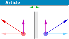
To use symmetry arguments we first need to establish how the magnetic field transforms under different spatial transformations. How it transforms under rotations and reflections will be of particular interest. The magnetic field is described by a vector $\vec B$ with both magnitude and direction. The component of a vector along the axis of rotation is preserved, while the component perpendicular to the axis rotates by the angle of the rotation, see Fig. 1. This is a property that is common for all vectors. However, there are two possibilities for how vectors under rotations can transform under reflections.

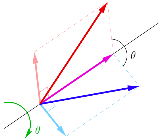
Figure 1. The red vector is rotated around the black axis by an angle $\theta$ into the blue vector. The component parallel to the axis (purple) is the same for both vectors. The component orthogonal to the axis (pink) is rotated by $\theta$ into the light blue component.

Let us look at the velocity vector $\vec v$ of an object through a reflecting mirror. The reflected object’s velocity appears to have the same components as the real object in the plane of the mirror. However, the component orthogonal to the mirror plane changes direction, see Fig. 2. We call vectors that behave in this fashion under reflections proper vectors, or just vectors.

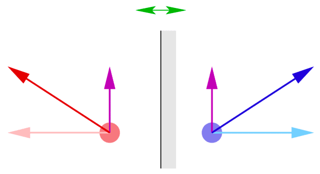
Figure 2. The velocity vector of a moving object (red) and its mirror image (blue) under a reflection in the black line. The component parallel to the mirror plane (purple) is the same for both. The component perpendicular to the mirror plane (pink) has its direction reversed for the reflection (light blue).

Transformation properties of axial vectors

A different type of vector is the angular velocity $\vec \omega$ of a solid. The angular velocity describes the rotation of the solid. It points in the direction of the rotational axis such that the object spins clockwise when looking in its direction, see Fig. 3. The magnitude of the angular velocity corresponds to the speed of the rotation.

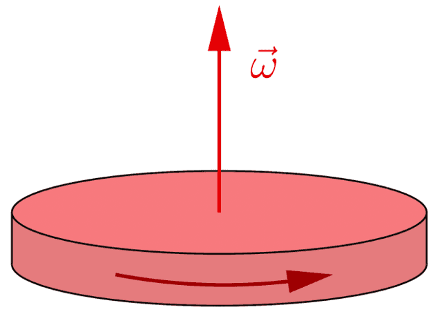
Figure 3. The angular velocity $\vec \omega$ of a spinning object. The spin direction is indicated by the darker red arrow.

So how does the angular velocity transform under reflections? Looking at an object spinning in the reflection plane, its mirror image will in the same direction. Therefore, unlike a proper vector, the component perpendicular to the mirror plane remains the same under reflections. At the same time, an object with an angular velocity parallel to the mirror plane will appear to have its spin direction reversed by the reflection. This means that the component parallel to the mirror plane changes sign, see Fig. 4. Overall, after a reflection, the angular velocity points in the exact opposite direction compared to if it were a proper vector. We call vectors that transform in this manner pseudo vectors or axial vectors.

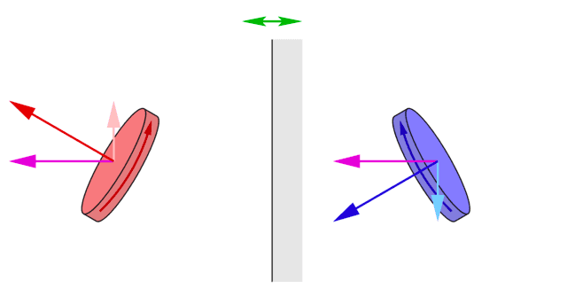
Figure 4. A rotating object (red) and its mirror image (blue) and their respective angular velocities. The components of the angular velocity perpendicular to the mirror plane (purple) are the same. The components parallel to the mirror plane (pink and light blue, respectively) are opposite in sign.

How does the magnetic field transform?

So what transformation rules does the magnetic field $\vec B$ follow? Is it a proper vector like a velocity or a pseudo-vector-like angular velocity?  In order to find out, let us consider Ampère’s law on integral form $$\oint_\Gamma \vec B \cdot d\vec x = \mu_0 \int_S \vec J \cdot d\vec S,$$ where $\mu_0$ is the permeability in vacuum, $\vec J$ the current density, $S$ an arbitrary surface, and $\Gamma$ the boundary curve of the surface. From the transformation properties of all of the other elements involved, we can deduce those of the magnetic field.

The surface normal of $S$ is such that the integration direction of $\Gamma$ is clockwise when looking in the direction of the normal. Performing a reflection for an arbitrary surface $S$, the displacements $d\vec x$ behave like a proper vector. In other words, the component orthogonal to the plane of reflection changes sign. Because of this, the components of surface element $d\vec S$ parallel to the plane of reflection must change sign. If this was not the case, then the relation between the surface normal and the direction of integration of the boundary curve would be violated. Therefore, the surface element $d\vec S$ is a pseudovector. We illustrate this in Fig. 5.

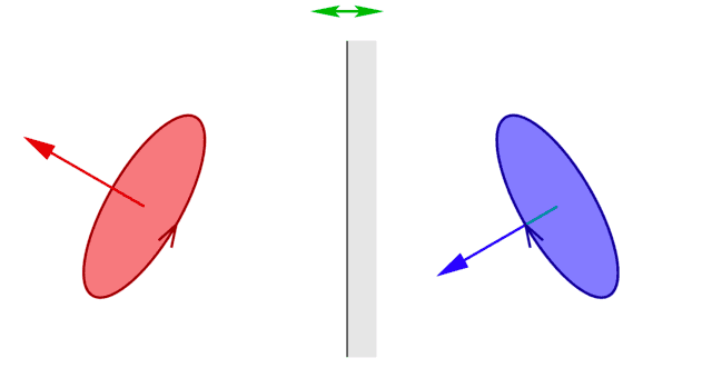
Figure 5. A surface element (red) and its mirror image (blue). The arrow on the boundary curves represents the direction of circulation. In order to keep the relation between the direction of circulation and the surface normal, the surface normal must transform into a pseudovector.

Finally, the current density $\vec J$ is a proper vector. If the current flows in the direction perpendicular to the mirror plane, then it will change direction under the reflection and if it is parallel to the mirror plane it will not. Consequently, the right-hand side of Ampère’s law changes sign under reflections since it contains an inner product between a proper vector and a pseudovector. If $\vec B$ was a proper vector, then the left-hand side would not change sign under reflections and Ampère’s law would no longer hold. The magnetic field $\vec B$ must therefore be a pseudovector.

What is a symmetry argument?

A symmetry of a system is a transformation that leaves the system the same. That a spherically symmetric charge distribution is not changed under rotations about its center is an example of this. However, the general form of physical quantities may not be the same after the transformation. If the solution for the quantity is unique, then it needs to be in a form that is the same before and after transformation. This type of reduction of the possible form of the solution is called a symmetry argument.

Symmetries of the current-carrying infinite wire

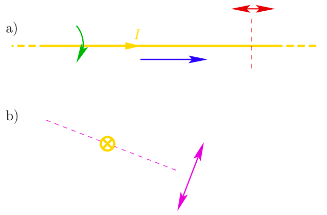
The infinite and straight wire with a current $I$ (see Fig. 6) has the following symmetries:

• Translations in the direction of the wire.
• Arbitrary rotations around the wire.
• Reflections in a plane containing the wire.
• Rotating the wire by an angle $\pi$ around an axis perpendicular to the wire while also changing the current direction.
  

  Figure 6. The infinite wire with a current $I$ is seen from the side (a) and with the current going into the page (b). The symmetries of the wire are translations in the wire direction (blue), rotations about the wire axis (green), and reflections in a plane containing the wire (magenta). Reflections in a plane perpendicular to the wire (red) are also a symmetry if the current direction is reversed at the same time as the reflection.

Any of the transformations above will leave an infinite straight wire carrying a current $I$ in the same direction. Since each individual transformation leaves the system the same, we can also perform combinations of these. This is a particular property of a mathematical construct called a group, but that is a story for another time.

The direction of the magnetic field

To find the direction of the magnetic field at a given point $p$ we only need a single transformation. This transformation is the reflection in a plane containing the wire and the point $p$, see Fig. 7. Since $\vec B$ is a pseudovector, its components in the direction of the wire and in the radial direction change sign under this transformation. However, the transformation is a symmetry of the wire and must therefore leave $\vec B$ the same. These components must therefore be equal to zero. On the other hand, the component in the tangential direction is orthogonal to the mirror plane. This component, therefore, retains its sign. Because of this, the reflection symmetry cannot say anything about it.

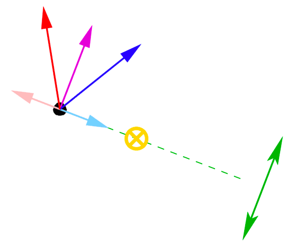
Figure 7. A reflection through a plane containing the wire and the black point $p$. Since the general magnetic field (red) is a pseudovector, it transforms to the blue field under the transformation. To be the same before and after the transformation, the component in the reflection plane (pink) needs to be zero. Only the component orthogonal to the reflection plane (purple) remains the same.

The magnitude of the magnetic field

The first two symmetries above can transform any points at the same distance $R$ into each other. This implies that the magnitude of the magnetic field can only depend on $R$. Using a circle of radius $R$ as the curve $\Gamma$ in Ampère’s law (see Fig. 8) we find $$\oint_\Gamma \vec B \cdot d\vec x = 2\pi R B = \mu_0 I$$ and therefore $$B = \frac{\mu_0 I}{2\pi R}.$$ Note that $\vec B \cdot d\vec x = BR\, d\theta$ since the magnetic field is parallel to $d\vec x$.

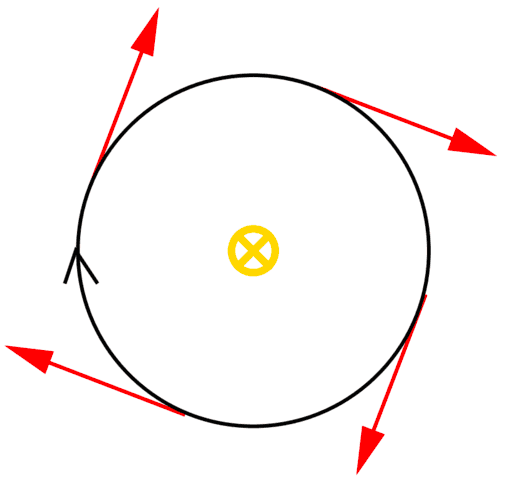
Figure 8. The integration curve $\Gamma$ (black) is used to compute the magnetic field strength. The curve is a distance $R$ from the wire and the red arrows represent the magnetic field along the curve.

Alternative to symmetry

For completeness, there is a more accessible way of showing that the radial component of the magnetic field is zero. This argument is based on Gauss’ law for magnetic fields $\nabla\cdot \vec B = 0$ and the divergence theorem.

We pick a cylinder of length $\ell$ and radius $R$ as our Gaussian surface and let its symmetry axis coincide with the wire. The surface integral over the end caps of the cylinder cancel as they have the same magnitude but opposite sign based on the translation symmetry. The integral over the side $S’$ of the cylinder becomes $$\int_{S’} \vec B \cdot d\vec S = \int_{S’} B_r\, dS = 2\pi R \ell B_r = 0.$$ The radial component $B_r$ appears as it is parallel to the surface normal. The zero on the right-hand side results from the divergence theorem $$\oint_S \vec B \cdot d\vec S = \int_V \nabla\cdot \vec B \, dV.$$ We conclude that $B_r = 0$.

While more accessible and seemingly simpler, this approach does not give us the result that the component in the wire direction is zero. Instead, we will need a separate argument for that. This is a bit more cumbersome and also not as satisfying as drawing both conclusions from a pure symmetry argument.