A New Interpretation of Dr. Walter Lewin’s Paradox

Much has lately been said regarding this paradox which first appeared in one of W. Lewin’s MIT lecture series on ##{YouTube}^{(1)}##.  This lecture was recently critiqued by C. Mabilde in a second YouTube video and submitted as a post in a PF ##{thread}^{(2)}##.  The latter cited the third source, that of K. T. McDonald of Princeton University, as support for Mabilde’s ##{presentation}^{(3)} {and}^{(4)}##.  Finally, Charles Link, PF Homework Helper, and Insight Author posted in Advisory Lounge Inner Circle (#1, May 25, 2018) on the same subject.  Furthermore, several other PF individuals (and probably others still)  have been involved in this topic.

I think a key concept, which none of the three sources mentions, is that there are two ##E## fields running around here.  One is the static field ##E_s## which by definition is conservative and the field lines of which begin and end on charges.  The second is the emf-induced field ##E_m## which is non-conservative in the sense that its circulation is non-zero.  ##E_m## can be created by a chemical battery, magnetic induction, the Seebeck effect, and others.

In the case of Faraday induction, its circulation is Faraday’s  ## \frac {-d\phi} {dt} ##. The two fields cancel each other in any loop wire segment but only ##E_s## exists in the resistors.  (This statement assumes negligible resistor body lengths and zero-resistance wires).  The net ##E## field is anywhere and everywhere just ## E = E_s + E_m ##, algebraically summed.

A voltmeter reads the line integral of ##E_s##, not any part of ##E_m##.

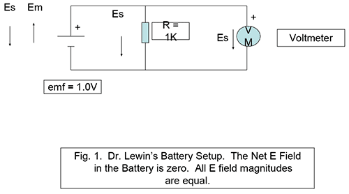
For example, in his battery setup  (Fig. 1) Dr. Lewin assumes a net battery ##E## field opposite to the direction of the ##E## field in the resistor.  Yet the battery has two canceling ##E## fields.  ##E_s## points + to – and ##E_m## points – to +. The line integral of ##E_m## over the length of the battery (- to +)  is the emf of the battery.  A voltmeter senses the line integral of ##E_s## only, otherwise the meter would read 0V DC.  The resistor has an ##E_s## field pointing + to -; the circulation of ##E_s## around the loop is zero as required by Kirchhoff’s voltage law.  The circulation of ##E_m##, and thus ##E##, is ##iR##, ##i## being the current and ##R## the resistor.*

Now to address the main topic here, that of the solenoid, the single-turn loop, and voltmeters positioned as shown in Fig. 2. In what follows, loop resistance is again assumed zero.

Let

##\phi## = magnetic flux inside loop,

loop radius =##a##

loop current = ##i##

total loop induced emf = ## \oint \bf E_m \cdot \bf dl ##

then $$ E_m = \frac {\frac {-d\phi} {dt}} {2\pi a}  $$.

Around the loop with or without the two resistors ##R1## and ##R2## in it, a continuum of ##E_m## field exists throughout the loop, with an ##E_s## field running in the opposite direction.

In the resistors ##E_s## can be very large as ## E_s = iR/d ##  with d the length of each resistor, ##d \ll {2\pi a} ##. All of this follows immediately from the realization that  ##\oint \vec E_s \cdot d \vec l = 0## and the line integral of the two resistors’ ##E_s## fields = ##\mathcal E##, being canceled around the loop by the wire segments’ ##E_s## fields.

Let us next show that a voltmeter as arranged in Fig. 3 and connected at two points a and b along the loop not including a resistor, reads 0V.  That this crucial fact is perhaps paradoxical but entirely logical can be shown as follows:

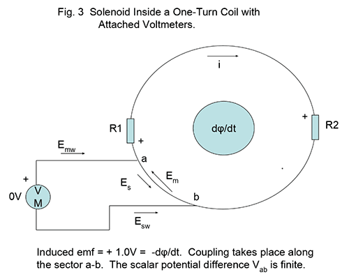
First, we remind ourselves that ##E_s## and ##E_m## are always equal and opposite in the wire including the shorter sections a-b, as well as in the meter leads since a perfect conductor cannot have a net E field.  This is a crucial assumption.

Let

##E_{mw}## = the static field in the meter leads ,

##E_{sw}## = the emf field in the meter leads,

##E_{sv}## = the static field  in the voltmeter,

##E_{mv}## =the emf  field int he voltmeter,

##l_w## = the total meter lead length,

We model the voltmeter as a resistor ##r## of finite physical length ##d##, of arbitrarily high resistance ##r## and passing correspondingly low current  ##i_v##  with the voltmeter reading ## i_v \cdot r####.

We must then also take cognizance of the fact that, for the voltmeter, ##i_v \cdot r  =  (E_{sv} – E_{mv}) \cdot d ## since ##E_{sv} ## and ##E_{mv} ## oppose. Thus, ##d \cdot E_{sv} = i \cdot r   +   d \cdot E_{mv} ##.

With this in mind, performing the circulation of ##E_s## around the meter circuit,

## +E_{sw} \cdot l_w   +  i_v \cdot r + E_{mv} \cdot d ~  –  ~ E_s\theta a  = 0 ##

The circulation of ##E_m## is also zero since there are no sources of emf within or around that contour:

## E_{mw} \cdot l_w + d \cdot E_{mv}  – E_m \theta a = 0 ##

Combining these last  two, with ##E_{sw} = E_{mw} ## and ##E_s = E_m ## as required,

##i_v\cdot r  = 0,  i_v = 0, VM = 0 ##.

Since VM = 0 for an uninterrupted section of the loop, it follows that the voltage read by a voltmeter probing a length of wire with a resistor ##R## in-between, VM = ##iR## and is not dependent on the length of wire segments surrounding ##R##. This argument includes of course Lewin’s famous A and D points which are located at the top and bottom respectively of the loop as in Figs. 2 or 3.

We thus distinguish between VM readings and the so-called “scalar potential” difference which is here ##\int \bf E_s \cdot \bf dl.##  McDonald rightly offers that meter wire coupling is accountable for the difference, which is why he argues for accepting scalar potential differences as the “true” potential difference, not subject to measurement detail.  This is also the explanation offered by Mr. Mabilde. The latter demonstrated a valid way of measuring the scalar potential experimentally with his interior voltage measuring setup, arriving at the correct scalar potential in all cases.  However, his demo is simply a simulation of the Es field profile around the ring, set up by the area of his meter leads.

His statement criticizing Lewin’s “Kirchhoff was wrong” is however spot-on if we understand that the Kirchhoff voltage law applies to voltages in the correct sense of the word, which is the line integral of the Es field only and does not apply to Em fields.

I want to emphasize that the voltmeter readings in Lewin’s setup can be entirely accounted for without splitting the E field into Em and Es.  What I think I contribute is more insight into the observed phenomena.   I believe I have offered a precise explanation for the difference between meter readings and scalar potential differences.  It’s not meter lead dress as suggested by Mr. Mabilde that matters; any meter loop in any orientation will give the same results.  It’s simply ##E_m## and ##E_s## sharing between loops.  As McDonald points out, if you want to avoid the consequences of loop coupling then the meter probes must be connected right at a resistor or the scalar potential difference reading will be wrong since those potentials associated with the loop wiring will not be included..

Lewin did not to my recollection place the VM leads in the middle of the solenoid.  I think we can all accept that the reading would be halfway between -0.1V and + 0.9V, i.e +0.4V.  Reflecting on the numerical mismatch between expected and actual VM readings, we see that the ##R1## meter reading was -0.1V – 0.4V = -0.5V i.e. too negative, while for the ##R2## loop, it was +0.9V – 0.4V = +0.5V (too positive).  Now, if we integrate the ##E_s## field over the meter loop with the meter positioned halfway, i.e. directly above, the solenoid, we can sum the line integral of ##E_s## as follows:

## \mathcal E##/2 – ##iR2##  +  VM = 0 or VM  = +0.4V.

Or,  –VM + ##\mathcal E##/2 –##iR1## = 0 also giving VM = +0.4V.  Which agrees with the data.  Suspending the voltmeter with its leads directly above the magnetic source gives the correct voltage.

To summarize, one should be aware of two separate electric fields in the loop and meter lead wiring vs. (essentially) one only in the resistors.  Voltmeters give erroneous voltage readings if the meter circuit forms an alternative path for the Em field, as it does in the Lewin setup and readings.    Coupling effects are predictable and can be shown to be ##E_m## and ##E_s## field sharing between the main loop and the meter loop.  Spurious coupling must be identified and avoided if one wishes to obtain actual scalar potential differences; this may not always be an easy task.

Failure to recognize the two types of ##E## field is bound to lead to confusion or even violation of physics laws in any circuit containing one or more sources of emf, be they batteries, magnetic induction, or any other form of emf generation.

Cf. Stanford Professor Emeritus H. H. Skilling, Fundamentals of Electric Waves, probably out of print but readily available on the Web.

References:

1. https://www.youtube.com/watch?v=FUUMCT7FjaI
2. https://www.physicsforums.com/threads/faradays-law-circular-loop-with-a-triangle.926206/page-4
3. Attachment: K. McDonald: “Lewin’s Circuit Paradox”
4. Attachment: K. McDonald, “What Does a Voltmeter Measure?”