Learn the Fields of Mathematical Quantum Field Theory
The following is one chapter in a series on Mathematical Quantum Field Theory
The previous chapter is 2. Spacetime.
The next chapter is 4. Field variations.
Table of Contents
3. Fields
A field history on a given spacetime ##\Sigma## (a history of spatial field configurations, see remark 3.2 below) is a quantity assigned to each point of spacetime (each event), such that this assignment varies smoothly with spacetime points. For instance, an electromagnetic field history (example 3.6 below) is at each point of spacetime a collection of vectors that encode the direction in which a charged particle passing through that point would feel a force (the “Lorentz force”, see example 3.6 below).
This is readily formalized (def. 3.1 below): If ##F## denotes the smooth manifold of “values” that the given kind of field may take at any spacetime point, then a field history ##\Phi## is modeled as a smooth function from spacetime to this space of values:
$$
\Phi
\;\colon\;
\Sigma
\longrightarrow
F
\,.
$$
It will be useful to unify spacetime and the space of field values (the field fiber) into a single manifold, the Cartesian product
$$
E \;:=\; \Sigma \times F
$$
and to think of this equipped with the projection map onto the first factor as a fiber bundle of spaces of field values over spacetime
$$
\array{
E &:=& \Sigma \times F
\\
{}^{\llap{fb}}\downarrow & \swarrow_{\rlap{pr_1}}
\\
\Sigma
}
\,.
$$
This is then called the field bundle, which specifies the kind of values that the given field species may take at any point of spacetime. Since the space ##F## of field values is the fiber of this fiber bundle (def. 1.9), it is sometimes also called the field fiber. (See also at fiber bundles in physics.)
Given a field bundle ##E \overset{fb}{\to}\Sigma##, then a field history is a section of that bundle (def. 1.7). The discussion of field theory concerns the space of all possible field histories, hence the space of sections of the field bundle (example 3.12 below). This is a very “large” generalized smooth space, called a diffeological space (def. 3.10 below).
Or rather, in the presence of fermion fields such as the Dirac field (example 3.50 below), the Pauli exclusion principle demands that the field bundle is a super-manifold and that the fermionic space of field histories (example 3.51 below) is a super-geometric generalized smooth space: a super smooth set (def. 3.40 below).
This smooth structure on the space of field histories will be crucial when we discuss observables of a field theory below because these are smooth functions on the space of field histories. In particular, it is this smooth structure that allows deriving that linear observables of a free field theory are given by distributions (prop. 7.5) below. Among these are the point evaluation observables (delta distributions) which are traditionally denoted by the same symbol as the field histories themselves.
Hence there are these aspects of the concept of “field” in physics, which are closely related, but crucially different:
aspects of the concept of fields
| aspect | term | type | description | def. |
| field component | ##\phi^a##, ##\phi^a_{,\mu}## | ##J^\infty_\Sigma(E) \to \mathbb{R}## | coordinate function on jet bundle of field bundle | def. 3.1, def. 4.1 |
| field history | ##\Phi##, ##\frac{\partial \Phi}{\partial x^\mu}## | ##\Sigma \to J^\infty_\Sigma(E)## | jet prolongation of section of field bundle | def. 3.1, def. 4.2 |
| field observable | ##\mathbf{\Phi}^a(x)##, ##\partial_{\mu} \mathbf{\Phi}^a(x), ## | ##\Gamma_{\Sigma}(E) \to \mathbb{R}## | derivatives of delta-functional on space of sections | def. 7.1, example 7.2 |
| averaging of field observable | ##\alpha^\ast \mapsto \underset{\Sigma}{\int} \alpha^\ast_a(x) \mathbf{\Phi}^a(x) \, dvol_\Sigma(x)## | ##\Gamma_{\Sigma,cp}(E^\ast) \to Obs(E_{scp},\mathbf{L})## | observable-valued distribution | def. 7.28 |
| algebra of quantum observables | ##\left( Obs(E,\mathbf{L})_{\mu c},\, \star\right)## | ##\mathbb{C}Alg## | non-commutative algebra structure on field observables | def. 14.9, def. 16.1 |
We now discuss these topics:
field bundles
Definition 3.1. (fields and field histories)
Given a spacetime ##\Sigma##, then a type of fields on ##\Sigma## is a smooth fiber bundle (def. 1.9)
$$
\array{E \\ \downarrow^{\rlap{fb}} \\ \Sigma }
$$
called the field bundle,
Given a type of fields on ##\Sigma## this way, then a field history of that type on ##\Sigma## is a term of that type, hence is a smooth section (def. 1.7) of this bundle, namely a smooth function of the form
$$
\Phi \;\colon\; \Sigma \longrightarrow E
$$
such that composed with the projection map it is the identity function, i.e. such that
$$
fb \circ \Phi = id
\phantom{AAAAAAA}
\array{
&& E
\\
& {}^{\llap{\Phi}}\nearrow & \downarrow^{\rlap{fb}}
\\
\Sigma & = & \Sigma
}
\,.
$$
The set of such sections/field histories is to be denoted
| $$ \label{SetOfFieldHistories} \Gamma_\Sigma(E) \;:=\; \left\{ \array{ && E \\ & {}^{\llap{\Phi}}\nearrow & \downarrow^{\rlap{fb}} \\ \Sigma &=& \Sigma } \phantom{fb} \right\} $$ | (18) |
Remark 3.2. (field histories are histories of spatial field configurations)
Given a section ##\Phi \in \Gamma_\Sigma(E)## of the field bundle (def. 3.1) and given a spacelike (def. 2.34) submanifold ##\Sigma_p \hookrightarrow \Sigma## (def. 3.34) of spacetime in codimension 1, then the restriction ##\Phi\vert_{\Sigma_p}## of ##\Phi## to ##\Sigma_p## may be thought of as a field configuration in space. As different spatial slices ##\Sigma_p## are chosen, one obtains such field configurations at different times. It is in this sense that the entirety of a section ##\Phi \in \Gamma_\Sigma(E)## is a history of field configurations, hence a field history (def 3.1).
Remark 3.3. (possible field histories)
After we give the set ##\Gamma_\Sigma(E)## of field histories (18) differential geometric structure, below in example 3.12 and example 3.46, we call it the space of field histories. This should be read as a space of possible field histories; containing all field histories that qualify as being of the type specified by the field bundle ##E##.
After we obtain equations of motion below in def. 5.22, these serve as the “laws of nature” that field histories should obey, and they define the subspace of those field histories that do solve the equations of motion; this will be denoted
$$
\Gamma_\Sigma(E)_{\delta_{EL}\mathbf{L}= 0}
\overset{\phantom{AAA}}{\hookrightarrow}
\Gamma_\Sigma(E)
$$
and called the on-shell space of field histories (40).
For the time being, not to get distracted from the basic idea of quantum field theory, we will focus on the following simple special case of field bundles:
Example 3.4. (trivial vector bundle as a field bundle)
In applications, the field fiber ##F = V## is often a finite-dimensional vector space. In this case, the trivial field bundle with fiber ##F## is of course a trivial vector bundle (def. 1.10).
Choosing any linear basis ##(\phi^a)_{a = 1}^s## of the field fiber, then over Minkowski spacetime (def. 2.17) we have canonical coordinates on the total space of the field bundle
$$
( (x^\mu), ( \phi^a ) )
\,,
$$
where the index ##\mu## ranges from ##0## to ##p##, while the index ##a## ranges from 1 to ##s##.
If this trivial vector bundle is regarded as a field bundle according to def. 3.1, then a field history ##\Phi## is equivalently an ##s##-tuple of real-valued smooth functions ##\Phi^a \colon \Sigma \to \mathbb{R}## on spacetime:
$$
\Phi = ( \Phi^a )_{a = 1}^s
\,.
$$
Example 3.5. (field bundle for real scalar field)
If ##\Sigma## is a spacetime and if the field fiber
$$
F := \mathbb{R}
$$
is simply the real line, then the corresponding trivial field bundle (def. 3.1)
$$
\array{
\Sigma \times \mathbb{R}
\\
{}^{\llap{pr_1}}\downarrow
\\
\Sigma
}
$$
is the trivial real line bundle (a special case of example 3.4) and the corresponding field type (def. 3.1) is called the real scalar field on ##\Sigma##. A configuration of this field is simply a smooth function on ##\Sigma## with values in the real numbers:
| $$ \label{SpaceOfFieldHistoriesOfRealScalarField} \Gamma_\Sigma(\Sigma \times \mathbb{R}) \;\simeq\; C^\infty(\Sigma) \,. $$ | (19) |
Example 3.6. (field bundle for electromagnetic field)
On Minkowski spacetime ##\Sigma## (def. 2.17), let the field bundle (def. 3.1) be given by the cotangent bundle
$$
E := T^\ast \Sigma
\,.
$$
This is a trivial vector bundle (example 3.4) with canonical field coordinates ##(a_\mu)##.
A section of this bundle, hence a field history, is a differential 1-form
$$
A \in \Gamma_\Sigma(T^\ast \Sigma) = \Omega^1(\Sigma)
$$
on spacetime (def. 1.16). Interpreted as a field history of the electromagnetic field on ##\Sigma##, this is often called the vector potential. Then the de Rham differential (def. 1.19) of the vector potential is a differential 2-form
$$
F := d A
$$
known as the Faraday tensor. In the canonical coordinate basis 2-forms this may be expanded as
| $$ \label{TensorFaraday} F = \underset{i = 1}{\overset{p}{\sum}} E_i d x^0 \wedge d x^i + \underset{1 \leq i \lt j \leq p}{\sum} B_{i j} d x^i \wedge d x^j \,. $$ | (20) |
Here ##(E_i)_{i = 1}^p## are called the components of the electric field, while ##(B_{i j})## are called the components of the magnetic field.
Example 3.7. (field bundle for Yang-Mills field over Minkowski spacetime)
Let ##\mathfrak{g}## be a Lie algebra of finite dimension with linear basis ##(t_\alpha)##, in terms of which the Lie bracket is given by
| $$ \label{LieAlgebraStructureConstants} [t_\alpha, t_\beta] \;=\; C^\gamma{}_{\alpha \beta} t_\gamma \,. $$ | (21) |
Over Minkowski spacetime ##\Sigma## (def. 2.17), consider then the field bundle which is the cotangent bundle tensored with the Lie algebra ##\mathfrak{g}##
$$
E := T^\ast \Sigma \otimes \mathfrak{g}
\,.
$$
This is the trivial vector bundle (example 3.4) with induced field coordinates
$$
( a_\mu^\alpha )
\,.
$$
A section of this bundle is a Lie algebra-valued differential 1-form
$$
A \in \Gamma_\Sigma(T^\ast \Sigma \otimes \mathfrak{g}) = \Omega^1(\Sigma, \mathfrak{g})
\,.
$$
with components
$$
A^\ast(a_\mu^\alpha) = A^\alpha_\mu
\,.
$$
This is called a field history for Yang-Mills gauge theory (at least if ##\mathfrak{g}## is a semisimple Lie algebra, see example (42) below).
For ##\mathfrak{g} = \mathbb{R}## is the line Lie algebra, this reduces to the case of the electromagnetic field (example 3.6).
For ##\mathfrak{g} = \mathfrak{su}(3)## this is a field history for the gauge field of the strong nuclear force in quantum chromodynamics.
For readers familiar with the concepts of principal bundles and connections on a bundle we include the following example 3.8 which generalizes the Yang-Mills field over Minkowski spacetime from example 3.7
to the situation over general spacetimes.
Example 3.8. (general Yang-Mills field in fixed topological sector)
Let ##\Sigma## be any spacetime manifold and let ##G## be a compact Lie group with Lie algebra denoted ##\mathfrak{g}##. Let ##P \overset{is}{\to} \Sigma## be a ##G##-principal bundle and ##\nabla_0## a chosen connection on it, to be called the background ##G##-Yang-Mills field.
Then the field bundle (def. 3.1) for ##G##-Yang-Mills theory in the topological sector ##P## is the tensor product of vector bundles
$$
E := \left(P \times^{ad}_G \mathfrak{g}\right) \otimes_\Sigma \left( T^\ast \Sigma \right)
$$
of the adjoint bundle of ##P## and the cotangent bundle of ##\Sigma##.
With the choice of ##\nabla_0##, every (other) connection ##\nabla## on ##P## uniquely decomposes as
$$
\nabla = \nabla_0 + A
\,,
$$
where
$$
A \in \Gamma_\Sigma(E)
$$
is a section of the above field bundle, hence a Yang-Mills field.
The electromagnetic field (def. 3.6) and the Yang-Mills field (def. 3.7, def. 3.8) with differential 1-forms as field histories are the basic examples of gauge fields (we consider this in more detail below in Gauge symmetries). There are also higher gauge fields with differential n-forms as field histories:
Example 3.9. (field bundle for B-field)
On Minkowski spacetime ##\Sigma## (def. 2.17), let the field bundle (def. 3.1) be given by the skew-symmetrized tensor product of vector bundles of the cotangent bundle with itself
$$
E := \wedge^2_\Sigma T^\ast \Sigma
\,.
$$
This is a trivial vector bundle (example 3.4) with canonical field coordinates ##(b_{\mu \nu})## subject to
$$
b_{\mu \nu} \;=\; – b_{\nu \mu}
\,.
$$
A section of this bundle, hence a field history, is a differential 2-form (def. 1.18)
$$
B \in \Gamma_\Sigma(\wedge^2_\Sigma T^\ast \Sigma) = \Omega^2(\Sigma)
$$
on spacetime.
space of field histories
Given any field bundle, we will eventually need to regard the set of all field histories ##\Gamma_\Sigma(E)## as a “smooth set” itself, a smooth space of sections, to which constructions of differential geometry apply (such as for the discussion of observables and states below ). Notably, we need to be talking about differential forms on ##\Gamma_\Sigma(E)##.
However, a space of sections ##\Gamma_\Sigma(E)## does not, in general, carry the structure of a smooth manifold; and it carries the correct smooth structure of an infinite-dimensional manifold only if ##\Sigma## is a compact space (see at the manifold structure of mapping spaces). Even if it does carry infinite-dimensional manifold structure, inspection shows that this is more structure than actually needed for the discussion of field theory. Namely, it turns out below that all we need to know is what counts as a smooth family of sections/field histories, hence which functions of sets
$$
\Phi_{(-)} \;\colon\; \mathbb{R}^n \longrightarrow \Gamma_\Sigma(E)
$$
from any Cartesian space ##\mathbb{R}^n## (def. 1.1) into ##\Gamma_\Sigma(E)## count as smooth functions, subject to some basic consistency condition on this choice.
This structure on ##\Gamma_\Sigma(E)## is called the structure of a diffeological space:
Definition 3.10. (diffeological space)
A diffeological space ##X## is
- a set ##X_s \in ## Set;
- for each ##n \in \mathbb{N}## a choice of subset$$
X(\mathbb{R}^n) \subset Hom_{Set}(\mathbb{R}^n_s, X_s) = \left\{ \mathbb{R}^n_s \to X_s \right\}
$$of the set of functions from the underlying set ##\mathbb{R}^n_s## of ##\mathbb{R}^n## to ##X_s##, to be called the smooth functions or plots from ##\mathbb{R}^n## to ##X##; - for each smooth function ##f \;\colon\; \mathbb{R}^{n_1} \longrightarrow \mathbb{R}^{n_2}## between Cartesian spaces (def. 1.1) a choice of function$$
f^\ast \;\colon\; X(\mathbb{R}^{n_2}) \longrightarrow X(\mathbb{R}^{n_1})
$$to be thought of as the precomposition operation$$
\left(
\mathbb{R}^{n_2} \overset{\Phi}{\longrightarrow} X
\right)
\;\overset{f^\ast}{\mapsto}\;
\left(
\mathbb{R}^{n_1} \overset{f}{\to} \mathbb{R}^{n_2} \overset{\Phi}{\to} X
\right)
$$
such that
- (constant functions are smooth)$$
X(\mathbb{R}^0) = X_s
\,,
$$ - (functionality)
- If ##id_{\mathbb{R}^n} \;\colon\; \mathbb{R}^n \to \mathbb{R}^n## is the identity function on ##\mathbb{R}^n##, then ##\left(id_{\mathbb{R}^n}\right)^\ast \;\colon\; X(\mathbb{R}^n) \to X(\mathbb{R}^n)## is the identity function on the set of plots ##X(\mathbb{R}^n)##;
- If ##\mathbb{R}^{n_1} \overset{f}{\to} \mathbb{R}^{n_2} \overset{g}{\to} \mathbb{R}^{n_3}## are two composable smooth functions between Cartesian spaces (def. 1.1), then pullback of plots along them consecutively equals the pullback along the composition:$$
f^\ast \circ g^\ast
=
(g \circ f)^\ast
$$i.e.$$
\array{
&& X(\mathbb{R}^{n_2})
\\
& {}^{\llap{f^\ast}}\swarrow && \nwarrow^{\rlap{g^\ast}}
\\
X(\mathbb{R}^{n_1})
&& \underset{ (g \circ f)^\ast }{\longleftarrow} &&
X(\mathbb{R}^{n_3})
}
$$
- (gluing)If ##\{ U_i \overset{f_i}{\to} \mathbb{R}^n\}_{i \in I}## is a differentiably good open cover of a Cartesian space (def. 1.5) then the function which restricts ##\mathbb{R}^n##-plots of ##X## to a set of ##U_i##-plots$$
X(\mathbb{R}^n)
\overset{( (f_i)^\ast )_{i \in I} }{\hookrightarrow}
\underset{i \in I}{\prod} X(U_i)
$$is a bijection onto the set of those tuples ##(\Phi_i \in X(U_i))_{i \in I}## of plots, which are “matching families” in that they agree on intersections:$$
\phi_i\vert_{U_i \cap U_j} = \phi_j \vert_{U_i \cap U_j}
\phantom{AAAAAA}
\array{
&& U_i \cap U_j
\\
& \swarrow && \searrow
\\
U_i && && U_j
\\
& {}_{\rlap{\Phi_i}}\searrow && \swarrow_{\rlap{\Phi_j}}
\\
&& X
}
$$
Finally, given ##X_1## and ##X_2## two diffeological spaces, then a smooth function between them
$$
f \;\colon\; X_1 \longrightarrow X_2
$$
is
- a function of the underlying sets$$
f_s \;\colon\; (X_1)_s \longrightarrow (X_2)_s
$$
such that
- for ##\Phi \in X(\mathbb{R}^n)## a plot of ##X_1##, then the composition ##f_s \circ \Phi_s## is a plot ##f_\ast(\Phi)## of ##X_2##:$$
\array{
&& \mathbb{R}^n
\\
& {}^{\llap{\Phi}}\swarrow && \searrow^{\rlap{f_\ast(\Phi)}}
\\
X_1 && \underset{f}{\longrightarrow} && X_2
}
\,.
$$
(Stated more abstractly, this says simply that diffeological spaces are the concrete sheaves on the site of Cartesian spaces from def. 1.5.)
For more background on diffeological spaces see also the geometry of physics — smooth sets.
Example 3.11. (Cartesian spaces are diffeological spaces)
Let ##X## be a Cartesian space (def. 1.1) Then it becomes a diffeological space (def. 3.10) by declaring its plots ##\Phi \in X(\mathbb{R}^n)## to the ordinary smooth functions ##\Phi \colon \mathbb{R}^n \to X##.
Under this identification, a function ##f \;\colon\; (X_1)_s \to (X_2)_s## between the underlying sets of two Cartesian spaces is a smooth function in the ordinary sense precisely if it is a smooth function in the sense of diffeological spaces.
Stated more abstractly, this statement is an example of the Yoneda embedding over a subcanonical site.
More generally, the same construction makes every smooth manifold a smooth set.
Example 3.12. (diffeological space of field histories)
Let ##E \overset{fb}{\to} \Sigma## be a smooth field bundle (def. 3.1). Then the set ##\Gamma_\Sigma(E)## of field histories/sections (def. 3.1) becomes a diffeological space (def. 3.10)
| $$ \label{SpaceOfFieldHistories} \Gamma_\Sigma(E) \in DiffeologicalSpaces $$ | (22) |
by declaring that a smooth family ##\Phi_{(-)}## of field histories, parameterized over any Cartesian space ##U## is a smooth function out of the Cartesian product manifold of ##\Sigma## with ##U##
$$
\array{
U \times \Sigma &\overset{\Phi_{(-)}(-)}{\longrightarrow}& E
\\
(u,x) &\mapsto& \Phi_u(x)
}
$$
such that for each ##u \in U## we have ##p \circ \Phi_{u}(-) = id_\Sigma##, i.e.
$$
\array{
&& E
\\
& {}^{\llap{\Phi_{(-)}(-)}}\nearrow & \downarrow^{\rlap{fb}}
\\
U \times \Sigma &\underset{pr_2}{\longrightarrow}& \Sigma
}
\,.
$$
The following example 3.13 is included only for readers who wonder how infinite-dimensional manifolds fit in. Since we will never actually use infinite-dimensional manifold structure, this example is may be ignored.
Example 3.13. (Fréchet manifolds are diffeological spaces)
Consider the particular type of infinite-dimensional manifolds called Fréchet manifolds. Since ordinary smooth manifolds ##U## is an example, for ##X## a Fréchet manifold there is a concept of smooth functions ##U \to X##. Hence we may give ##X## the structure of a diffeological space (def. 3.10) by declaring the plots over ##U## to be these smooth functions ##U \to X##, with the evident post-composition action.
It turns out that then that for ##X## and ##Y## two Fréchet manifolds, there is a natural bijection between the smooth functions ##X \to Y## between them regarded as Fréchet manifolds and [regarded as diffeological spaces. Hence it does not matter which of the two perspectives we take (unless of course, a diffeological space more general than a Fréchet manifold enters the picture, at which point the second definition generalizes, whereas the first does not).
Stated more abstractly, this means that Fréchet manifolds form a full subcategory of that of diffeological spaces (this prop.):
$$
FrechetManifolds \hookrightarrow DiffeologicalSpaces
\,.
$$
If ##\Sigma## is a compact smooth manifold and ##E \simeq \Sigma \times F \to \Sigma## is a trivial fiber bundle with fiber ##F## a smooth manifold, then the set of sections ##\Gamma_\Sigma(E)## carries a standard structure of a Fréchet manifold (see at manifold structure of mapping spaces). Under the above inclusion of Fréchet manifolds into diffeological spaces, this smooth structure agrees with that from example 3.12 (see this prop.)
Once the step from smooth manifolds to diffeological spaces (def. 3.10) is made, characterizing the smooth structure of the space entirely by how we may probe it by mapping smooth Cartesian spaces into it, it becomes clear that the underlying set ##X_s## of a diffeological space ##X## is not actually crucial to support the concept: The space is already entirely defined structurally by the system of smooth plots it has, and the underlying set ##X_s## is recovered from these as the set of plots from the point ##\mathbb{R}^0##.
This is crucial for field theory: the spaces of field histories of fermionic fields (def. 3.45 below) such as the Dirac field (example 3.51 below) do not have underlying sets of points the way diffeological spaces have. Informally, the reason is that a point is a bosonic object, while and the nature of fermionic fields is the opposite of bosonic.
But we may just as well drop the mentioning of the underlying set ##X_s## in the definition of generalized smooth spaces. By simply stripping this requirement off of def. 3.10 we obtain the following more general and more useful definition (still “bosonic”, though, the supergeometric version is def. 3.40 below):
Definition 3.14. (smooth set)
A smooth set ##X## is
- for each ##n \in \mathbb{N}## a choice of set$$
X(\mathbb{R}^n) \in Set
$$to be called the set of smooth functions or plots from ##\mathbb{R}^n## to ##X##; - for each smooth function ##f \;\colon\; \mathbb{R}^{n_1} \longrightarrow \mathbb{R}^{n_2}## between Cartesian spaces a choice of function$$
f^\ast \;\colon\; X(\mathbb{R}^{n_2}) \longrightarrow X(\mathbb{R}^{n_1})
$$to be thought of as the precomposition operation$$
\left(
\mathbb{R}^{n_2} \overset{\Phi}{\longrightarrow} X
\right)
\;\overset{f^\ast}{\mapsto}\;
\left(
\mathbb{R}^{n_1} \overset{f}{\to} \mathbb{R}^{n_2} \overset{\Phi}{\to} X
\right)
$$
such that
- (functionality)
- If ##id_{\mathbb{R}^n} \;\colon\; \mathbb{R}^n \to \mathbb{R}^n## is the identity function on ##\mathbb{R}^n##, then ##\left(id_{\mathbb{R}^n}\right)^\ast \;\colon\; X(\mathbb{R}^n) \to X(\mathbb{R}^n)## is the identity function on the set of plots ##X(\mathbb{R}^n)##.
- If ##\mathbb{R}^{n_1} \overset{f}{\to} \mathbb{R}^{n_2} \overset{g}{\to} \mathbb{R}^{n_3}## are two composable smooth functions between Cartesian spaces, then consecutive pullback of plots along them equals the pullback along the composition:$$
f^\ast \circ g^\ast
=
(g \circ f)^\ast
$$i.e.$$
\array{
&& X(\mathbb{R}^{n_2})
\\
& {}^{\llap{f^\ast}}\swarrow && \nwarrow^{\rlap{g^\ast}}
\\
X(\mathbb{R}^{n_1})
&& \underset{ (g \circ f)^\ast }{\longleftarrow} &&
X(\mathbb{R}^{n_3})
}
$$
- (gluing)If ##\{ U_i \overset{f_i}{\to} \mathbb{R}^n\}_{i \in I}## is a differentiably good open cover of a Cartesian space (def. 1.5) then the function which restricts ##\mathbb{R}^n##-plots of ##X## to a set of ##U_i##-plots$$
X(\mathbb{R}^n)
\overset{( (f_i)^\ast )_{i \in I} }{\hookrightarrow}
\underset{i \in I}{\prod} X(U_i)
$$is a bijection onto the set of those tuples ##(\Phi_i \in X(U_i))_{i \in I}## of plots, which are “matching families” in that they agree on intersections:$$
\phi_i\vert_{U_i \cap U_j} = \phi_j \vert_{U_i \cap U_j}
\phantom{AAAA}
\text{i.e.}
\phantom{AAAA}
\array{
&& U_i \cap U_j
\\
& \swarrow && \searrow
\\
U_i && && U_j
\\
& {}_{\rlap{\Phi_i}}\searrow && \swarrow_{\rlap{\Phi_j}}
\\
&& X
}
$$
Finally, given ##X_1## and ##X_2## two smooth sets, then a smooth function between them
$$
f \;\colon\; X_1 \longrightarrow X_2
$$
is
- for each ##n \in \mathbb{N}## a function$$
f_\ast(\mathbb{R}^n)
\;\colon\;
X_1(\mathbb{R}^n) \longrightarrow X_2(\mathbb{R}^n)
$$
such that
- for each smooth function ##g \colon \mathbb{R}^{n_1} \to \mathbb{R}^{n_2}## between Cartesian spaces we have$$
g^\ast_2 \circ f_\ast(\mathbb{R}^{n_2})
=
f_\ast(\mathbb{R}^{n_1}) \circ g^\ast_1
\phantom{AAAAA}
\text{i.e.}
\phantom{AAAAA}
\text{i.e.}
\phantom{AAAAA}
\array{
X_1(\mathbb{R}^{n_2})
&\overset{f_\ast(\mathbb{R}^{n_2})}{\longrightarrow}&
X_2(\mathbb{R}^{n_2})
\\
\llap{g_1^\ast}\downarrow && \downarrow\rlap{g^\ast_2}
\\
X_1(\mathbb{R}^{n_1})
&\underset{f_\ast(\mathbb{R}^{n_1})}{\longrightarrow}&
X_2(\mathbb{R}^{n_1})
}
$$
Stated more abstractly, this simply says that smooth sets are the _sheaves on the site of Cartesian spaces from def. 1.5.
Basing differential geometry on smooth sets is an instance of the general approach to geometry called functorial geometry or topos theory. For more background on this see at geometry of physics — smooth sets.
First we verify that the concept of smooth sets is a consistent generalization:
Example 3.15. (diffeological spaces are smooth sets)
Every diffeological space ##X## (def. 3.10) is a smooth set (def. 3.14) simply by forgetting its underlying set of points and remembering only its sets of plot.
In particular therefore each Cartesian space ##\mathbb{R}^n## is canonically a smooth set by example 3.11.
Moreover, given any two diffeological spaces, then the morphisms ##f \colon X \to Y## between them, regarded as diffeological spaces, are the same as the morphisms as smooth sets.
Stated more abstractly, this means that we have full subcategory inclusions
$$
CartesianSpaces
\overset{\phantom{AAA}}{\hookrightarrow}
DiffeologicalSpaces
\overset{\phantom{AAA}}{\hookrightarrow}
SmoothSets
\,.
$$
Recall, for the next proposition 3.16, that in the definition 3.14 of a smooth set ##X## the sets ##X(\mathbb{R}^n)## are abstract sets which are to be thought of as would-be smooth functions “##\mathbb{R}^n \to X##”. Inside def. 3.14 this only makes sense in quotation marks, since inside that definition the smooth set ##X## is only being defined, so that inside that definition there is not yet an actual concept of smooth functions of the form “##\mathbb{R}^n \to X##”.
But now that the definition of smooth sets and of morphisms between them has been stated, and seeing that Cartesian space ##\mathbb{R}^n## are examples of smooth sets, by example 3.15, there is now an actual concept of smooth functions ##\mathbb{R}^n \to X##, namely as smooth sets. For the concept of smooth sets to be consistent, it ought to be true that this a posteriori concept of smooth functions from Cartesian spaces to smooth sets coincides with the a priori concept, hence that we “may remove the quotation marks” in the above. The following proposition says that this is indeed the case:
Proposition 3.16. (plots of a smooth set really are the smooth functions into the smooth set)
Let ##X## be a smooth set (def. 3.14). For ##n \in \mathbb{R}##, there is a natural function
$$
Hom_{SmoothSet}(\mathbb{R}^n , X) \overset{\phantom{AA}\simeq\phantom{AA}}{\longrightarrow} X(\mathbb{R}^n)
$$
from the set of homomorphisms of smooth sets from ##\mathbb{R}^n## (regarded as a smooth set via example 3.15) to ##X##, to the set of plots of ##X## over ##\mathbb{R}^n##, given by evaluating on the identity plot ##id_{\mathbb{R}^n}##.
This function is a bijection.
This says that the plots of ##X##, which initially bootstrap ##X## into being as declaring the would-be smooth functions into ##X##, end up being the actual smooth functions into ##X##.
Proof. This elementary but profound fact is called the Yoneda lemma, here in its incarnation over the site of Cartesian spaces (def. 1.1).
A key class of examples of smooth sets (def. 3.14) that are not diffeological spaces (def. 3.10) are universal smooth moduli spaces of differential forms:
Example 3.17. (universal smooth moduli spaces of differential forms)
For ##k \in \mathbb{N}## there is a smooth set (def. 3.14)
$$
\mathbf{\Omega}^k \;\in\; SmoothSet
$$
defined as follows:
- for ##n \in \mathbb{N}## the set of plots from ##\mathbb{R}^n## to ##\mathbf{\Omega}^k## is the set of smooth differential k-forms on ##\mathbb{R}^n## (def. 1.18)$$
\mathbf{\Omega}^k(\mathbb{R}^n) \;:=\; \Omega^k(\mathbb{R}^n)
$$ - for ##f \colon \mathbb{R}^{n_1} \to \mathbb{R}^{n_2}## a smooth function (def. 1.1) the operation of fullback of plots along ##f## is just the pullback of differential forms ##f^\ast## from prop. 1.21
$$
\array{
\mathbb{R}^{n_1} && \Omega^k(\mathbb{R}^{n_1})
\\
\downarrow^{\rlap{f}} && \uparrow^{\rlap{f^\ast}}
\\
\mathbb{R}^{n_2} && \Omega^k(\mathbb{R}^{n_2})
}
$$
That this is functorial is just the standard fact (7) from prop. 1.21.
For ##k = 1## the smooth set ##\mathbf{\Omega}^0## actually is a diffeological space, in fact under the identification of example 3.15 this is just the real line:
$$
\mathbf{\Omega}^0 \simeq \mathbb{R}^1
\,.
$$
But for ##k \geq 1## we have that the set of plots on ##\mathbb{R}^0 = \ast## is a singleton
$$
\mathbf{\Omega}^{k \geq 1}(\mathbb{R}^0) \simeq \{0\}
$$
consisting just of the zero differential form. The only diffeological space with this property is ##\mathbb{R}^0 = \ast## itself. But ##\mathbf{\Omega}^{k \geq 1}## is far from being that trivial: even though its would-be underlying set is a single point, for all ##n \geq k## it admits an infinite set of plots. Therefore the smooth sets ##\mathbf{\Omega}^k## for ##k \geq## are not diffeological spaces.
That the smooth set ##\mathbf{\Omega}^k## indeed deserves to be addressed as the universal moduli space of differential k-forms follows from prop. 3.16: The universal moduli space of ##k##-forms ought to carry a universal differential ##k##-forms ##\omega_{univ} \in \Omega^k(\mathbf{\Omega}^k)## such that every differential ##k##-form ##\omega## on any ##\mathbb{R}^n## arises as the pullback of differential forms of this universal one along some modulating morphism ##f_\omega \colon X \to \mathbf{\Omega}^k##:
$$
\array{
\{\omega\} &\overset{(f_\omega)^\ast}{\longleftarrow}& \{\omega_{univ}\}
\\
\\
X &\underset{f_\omega}{\longrightarrow}& \mathbf{\Omega}^k
}
$$
But with prop. 3.16 this is precisely what the definition of the plots of ##\mathbf{\Omega}^k## says.
Similarly, all the usual operations on differential form now have their universal archetype on the universal moduli spaces of differential forms
In particular, for ##k \in \mathbb{N}## there is a canonical morphism of smooth sets of the form
$$
\mathbf{\Omega}^k \overset{\mathbf{d}}{\longrightarrow} \mathbf{\Omega}^{k+1}
$$
defined over ##\mathbb{R}^n## by the ordinary de Rham differential (def. 1.19)
| $$ \label{deRhamDifferentialUniversal} \Omega^k(\mathbb{R}^n) \overset{d}{\longrightarrow} \Omega^{k+1}(\mathbb{R}^n) \,. $$ | (23) |
That this satisfies the compatibility with pre-composition of plots
$$
\array{
\mathbb{R}^{n_1} && \Omega^k(\mathbb{R}^{n_1}) &\overset{d}{\longrightarrow}& \Omega^{k+1}(\mathbb{R}^{n_1})
\\
{}^{\llap{f}}\downarrow && \uparrow^{\rlap{f^\ast}} && \uparrow^{\rlap{f^\ast}}
\\
\mathbb{R}^{n_2} && \Omega^k(\mathbb{R}^{n_2}) &\underset{d}{\longrightarrow}& \Omega^k( \mathbb{R}^{n_2} )
}
$$
is just the compatibility of pullback of differential forms with the de Rham differential of from prop. 1.21.
The upshot is that we now have a good definition of differential forms on any diffeological space and more generally on any smooth set:
Definition 3.18. (differential forms on smooth sets)
Let ##X## be a diffeological space (def. 3.10) or more generally a smooth set (def. 3.14) then a differential k-form ##\omega## on ##X## is equivalently a morphism of smooth sets
$$
X \longrightarrow \mathbf{\Omega}^k
$$
from ##X## to the universal smooth moduli space of differential froms from example 3.17.
Concretely, by unwinding the definitions of ##\mathbf{\Omega}^k## and of morphisms of smooth sets, this means that such a differential form is:
- for each ##n \in \mathbb{N}## and each plot ##\mathbb{R}^n \overset{\Phi}{\to} X## an ordinary differential form$$
\Phi^\ast(\omega) \in \Omega^\bullet(\mathbb{R}^n)
$$
such that
- for each smooth function ##f \;\colon\; \mathbb{R}^{n_1} \to \mathbb{R}^{n_2}## between Cartesian spaces the ordinary pullback of differential forms along ##f## is compatible with these choices, in that for every plot ##\mathbb{R}^{n_2} \overset{\Phi}{\to} X## we have$$
f^\ast\left(\Phi^\ast(\omega)\right)
=
( f^\ast \Phi )^\ast(\omega)
$$i.e.$$
\array{
\mathbb{R}^{n_1} && \overset{f}{\longrightarrow} && \mathbb{R}^{n_2}
\\
& {}_{\llap{f^\ast \Phi}}\searrow && \swarrow_{\rlap{\Phi}}
\\
&& X
}
\phantom{AAAA}
\array{
\Omega^\bullet( \mathbb{R}^{n_1} ) && \overset{f^\ast}{\longleftarrow} && \Omega^\bullet(\mathbb{R}^{n_2})
\\
& {}_{\llap{(f^\ast \Phi)^\ast}}\nwarrow && \nearrow_{\rlap{\Phi^\ast}}
\\
&& \Omega^\bullet(X)
}
\,.
$$
We write ##\Omega^\bullet(X)## for the set of differential forms on the smooth set ##X## defined this way.
Moreover, given a differential k-form
$$
X \overset{\omega}{\longrightarrow} \mathbf{\Omega}^k
$$
on a smooth set ##X## this way, then its de Rham differential ##d \omega \in \Omega^{k+1}(X)## is given by the composite of morphisms of smooth sets with the universal de Rham differential from (23):
| $$ \label{FormsOnSmoothSetDeRhamDifferential} d \omega \;\colon\; X \overset{\omega}{\longrightarrow} \mathbf{\Omega}^k \overset{d}{\longrightarrow} \mathbf{\Omega}^{k+1} \,. $$ | (24) |
Explicitly this means simply that for ##\Phi \colon U \to X## a plot, then
$$
\Phi^\ast (d\omega)
\;=\;
d\left( \Phi^\ast \omega\right)
\;\in\;
\Omega^{k+1}(U)
\,.
$$
The usual operations on ordinary differential forms directly generalize plot-wise to differential forms on diffeological spaces and more generally on smooth sets:
Definition 3.19. (exterior differential and exterior product on smooth sets)
Let ##X## be a diffeological space (def. 3.10) or more generally a smooth set (def. 3.14). Then
- For ##\omega \in \Omega^n(X)## a differential form on ##X## (def. 3.18) its exterior differential$$
d \omega \in \Omega^{n+1}(X)
$$is defined on any plot ##\mathbb{R}^n \overset{\Phi}{\to} X## as the ordinary exterior differential of the pullback of ##\omega## along that plot:$$
\Phi^\ast(d \omega) := d \Phi^\ast(\omega)
\,.
$$ - For ##\omega_1 \in \Omega^{n_1}## and ##\omega_2 \in \Omega^{n_2}(X)## two differential forms on ##X## (def. 3.18) then their exterior product$$
\omega_1 \wedge \omega_2 \;\in\; \Omega^{n_1 + n_2}(X)
$$is the differential form defined on any plot ##\mathbb{R}^n \overset{\Phi}{\to} X## as the ordinary exterior product of the pullback of th differential forms ##\omega_1## and ##\omega_2## to this plot:$$
\Phi^\ast(\omega_1 \wedge \omega_2)
\;:=\;
\Phi^\ast(\omega_1) \wedge \Phi^\ast(\omega_2)
\,.
$$
Infinitesimal geometry
It is crucial in field theory that we consider field histories not only over all of the spacetime but also restricted to submanifolds of spacetime. Or rather, what is actually of interest are the restrictions of the field histories to the infinitesimal neighborhoods (example 3.30 below) of these submanifolds. This appears notably in the construction of phase spaces below. Moreover, fermion fields such as the Dirac field (example 3.50 below) take values in graded infinitesimal spaces, called super spaces (discussed below). Therefore “infinitesimal geometry”, sometimes called formal geometry (as in “formal scheme”) or synthetic differential geometry or synthetic differential supergeometry, is a central aspect of field theory.
In order to mathematically grasp what infinitesimal neighborhoods are, we appeal to the first magic algebraic property of differential geometry from prop. 1.15, which says that we may recognize smooth manifolds ##X## dually in terms of their commutative algebras ##C^\infty(X)## of smooth functions on them
$$
C^\infty(-) \;\colon\; SmoothManifolds \overset{\phantom{AAA}}{\hookrightarrow} (\mathbb{R} Algebras)^{op}
\,.
$$
But since there are of course more algebras ##A \in \mathbb{R}Algebras## than arise this way from smooth manifolds, we may turn this around and try to regard any algebra ##A## as defining a would-be space, which would have ##A## as its algebra of functions.
For example, an infinitesimally thickened point should be a space that is “so small” that every smooth function ##f## on it which vanishes at the origin takes values so tiny that some finite power of them is not just even tinier, but actually vanishes:
Definition 3.20. (infinitesimally thickened Cartesian space)
An infinitesimally thickened point
$$
\mathbb{D} := Spec(A)
$$
is represented by a commutative algebra ##A \in \mathbb{R}Alg## which as real vector space is a direct sum
$$
A \simeq_{\mathbb{R}} \langle 1 \rangle \oplus V
$$
of the 1-dimensional space ##\langle 1 \rangle = \mathbb{R}## of multiples of 1 with a finite dimensional vector space ##V## that is a nilpotent ideal in that for each element ##a \in V## there exists a natural number ##n \in \mathbb{N}## such that
$$
a^{n+1} = 0
\,.
$$
More generally, an infinitesimally thickened Cartesian space
$$
\mathbb{R}^n \times \mathbb{D} \;:=\; \mathbb{R}^n \times Spec(A)
$$
is represented by a commutative algebra
$$
C^\infty(\mathbb{R}^n) \otimes A \;\in\; \mathbb{R} Alg
$$
which is the tensor product of algebras of the algebra of smooth functions ##C^\infty(\mathbb{R}^n)## on an actual Cartesian space of some dimension ##n## (example 1.3), with an algebra of functions ##A \simeq_{\mathbb{R}} \langle 1\rangle \oplus V## of an infinitesimally thickened point, as above.
We say that a smooth function between two infinitesimally thickened Cartesian spaces
$$
\mathbb{R}^{n_1} \times Spec(A_1) \overset{f}{\longrightarrow} \mathbb{R}^{n_2} \times Spec(A_2)
$$
is by definition dually an ##\mathbb{R}##-algebra homomorphism of the form
$$
C^\infty(\mathbb{R}^{n_1}) \otimes A_1
\overset{f^\ast}{\longleftarrow}
C^\infty(\mathbb{R}^{n_2}) \otimes A_2
\,.
$$
Example 3.21. (infinitesimal neighborhoods in the real line )
Consider the quotient algebra of the formal power series algebra ##\mathbb{R}[ [\epsilon] ]## in a single parameter ##\epsilon## by the ideal generated by ##\epsilon^2##:
$$
(\mathbb{R}[ [\epsilon] ])/(\epsilon^2)
\;\simeq_{\mathbb{R}}\;
\mathbb{R} \oplus \epsilon \mathbb{R}
\,.
$$
(This is sometimes called the algebra of dual numbers, for no good reason.) The underlying real vector space of this algebra is, as shown, the direct sum of the multiples of 1 with the multiples of ##\epsilon##. A general element in this algebra is of the form
$$
a + b \epsilon \in (\mathbb{R}[\epsilon])/(\epsilon^2)
$$
where ##a,b \in \mathbb{R}## are real numbers. The product in this algebra is given by “multiplying out” as usual, and discarding all terms proportional to ##\epsilon^2##:
$$
\left(
a_1 + b_1 \epsilon
\right)
\cdot
\left(
a_2 + b_2 \epsilon
\right)
\;=\;
a_1 a_2 + ( a_1 b_2 + b_1 a_2 ) \epsilon
\,.
$$
We may think of an element ##a + b \epsilon## as the truncation to the first order of a Taylor series at the origin of a smooth function on the real line
$$
f \;\colon\; \mathbb{R} \to \mathbb{R}
$$
where ##a = f(0)## is the value of the function at the origin, and where ##b = \frac{\partial f}{\partial x}(0)## is its first derivative at the origin.
Therefore this algebra behaves like the algebra of smooth function on an infinitesimal neighborhood ##\mathbb{D}^1## of ##0 \in \mathbb{R}## which is so tiny that its elements ##\epsilon \in \mathbb{D}^1 \hookrightarrow \mathbb{R}## become, upon squaring them, not just tinier, but actually zero:
$$
\epsilon^2 = 0
\,.
$$
This intuitive picture is now made precise by the concept of infinitesimally thickened points def. 3.20, if we simply set
$$
\mathbb{D}^1
\;:=\;
Spec\left(
\mathbb{R}[ [\epsilon] ]/(\epsilon^2)
\right)
$$
and observe that there is the inclusion of infinitesimally thickened Cartesian spaces
$$
\mathbb{D}^1 \overset{\phantom{AA}i\phantom{AA} }{\hookrightarrow} \mathbb{R}^1
$$
which is dually given by the algebra homomorphism
$$
\array{
\mathbb{R} \oplus \epsilon \mathbb{R}
&\overset{i^\ast}{\longleftarrow}&
C^\infty(\mathbb{R}^1)
\\
f(0) + \frac{\partial f}{\partial x}(0) &\longleftarrow& \{f\}
}
$$
which sends a smooth function to its value ##f(0)## at zero plus ##\epsilon## times its derivative at zero. Observe that this is indeed a homomorphism of algebras due to the product law of differentiation>, which says that
$$
\begin{aligned}
i^\ast(f \cdot g)
& =
(f \cdot g)(0) + \frac{\partial f \cdot g}{\partial x}(0) \epsilon
\\
& =
f(0) \cdot g(0)
+
\left(
\frac{\partial f}{\partial x}(0) \cdot g(0) + f(0) \cdot \frac{\partial g}{\partial x}(0)
\right) \epsilon
\\
& =
\left(
f(0) + \frac{\partial f}{\partial x}(0) \epsilon
\right)
\cdot
\left(
g(0) + \frac{\partial g}{\partial x}(0) \epsilon
\right)
\end{aligned}
$$
Hence we see that restricting a smooth function to the infinitesimal neighborhood of a point is equivalent to restricting attention to its [[Taylor series|] to the given order at that point:
$$
\array{
\mathbb{D}^1 &\overset{i}{\hookrightarrow}& \mathbb{R}^1
\\
& {}_{\llap{(\epsilon \mapsto f(0) + \frac{\partial f}{\partial x}(0) \epsilon) }}\searrow & \downarrow_{\rlap{f}}
\\
&& \mathbb{R}^1
}
$$
Similarly for each ##k \in \mathbb{N}## the algebra
$$
(\mathbb{R}[ [ \epsilon ] ])/(\epsilon^{k+1})
$$
may be thought of as the algebra of Taylor series at the origin of ##\mathbb{R}## of smooth functions ##\mathbb{R} \to \mathbb{R}##, where all terms of order higher than ##k## are discarded. The corresponding infinitesimally thickened point is often denoted
$$
\mathbb{D}^1(k) \;:=\; Spec\left( \left(\mathbb{R}[ [\epsilon] ]\right)/(\epsilon^{k+1}) \right)
\,.
$$
This is now the subobject of the real line
$$
\mathbb{D}^1(k) \overset{\phantom{AAA}}{\hookrightarrow} \mathbb{R}^1
$$
on those elements ##\epsilon## such that ##\epsilon^{k+1} = 0##.
(Kock 81, Kock 10)
The following example 3.22 shows that infinitesimal thickening is invisible for ordinary spaces when mapping out of these. In contrast example 3.23 further below shows that the morphisms into an ordinary space out of an infinitesimal space are interesting: these are tangent vectors and their higher-order infinitesimal analogs.
Example 3.22. (infinitesimal line ##\mathbb{D}^1## has a unique global point)
For ##\mathbb{R}^n## any ordinary Cartesian space (def. 1.1) and ##D^1(k) \hookrightarrow \mathbb{R}^1## the order-##k## infinitesimal neighborhood of the origin in the real line from example 3.21, there is exactly only one possible morphism of infinitesimally thickened Cartesian spaces from ##\mathbb{R}^n## to ##\mathbb{D}^1(k)##:
$$
\array{
\mathbb{R}^n && \overset{\exists !}{\longrightarrow} &6 \mathbb{D}^1(k)
\\
& {}_{\llap{\exists !}}\searrow && \nearrow_{\rlap{\exists !}}
\\
&& \mathbb{R}^0 = \ast
}
\,.
$$
Proof. By definition, such a morphism is dually an algebra homomorphism
$$
C^\infty(\mathbb{R}^n)
\overset{f^\ast}{\longleftarrow}
\left(
\mathbb{R}[ [\epsilon] ])/(\epsilon^{k+1}
\right)
\simeq_{\mathbb{R}}
\mathbb{R} \oplus \mathcal{O}(\epsilon)
$$
from the higher-order “algebra of dual numbers” to the algebra of smooth functions (example 1.3).
Now, this being an ##\mathbb{R}##-algebra homomorphism, its action on the multiples ##c \in \mathbb{R}## of the identity is fixed:
$$
f^\ast(1) = 1
\,.
$$
All the remaining elements are proportional to ##\epsilon##, and hence are nilpotent. However, by the homomorphism property of an algebra homomorphism it follows that it must send nilpotent elements ##\epsilon## to nilpotent elements ##f(\epsilon)##, because
$$
\begin{aligned}
\left(f^\ast(\epsilon)\right)^{k+1}
& = f^\ast\left( \epsilon^{k+1}\right)
\\
& = f^\ast(0)
\\ & = 0
\end{aligned}
$$
But the only nilpotent element in ##C^\infty(\mathbb{R}^n)## is the zero elements, and hence it follows that
$$
f^\ast(\epsilon) = 0
\,.
$$
Thus ##f^\ast## as above is uniquely fixed.
Example 3.23. (synthetic tangent vector fields)
Let ##\mathbb{R}^n## be a Cartesian space (def. 1.1), regarded as an infinitesimally thickened Cartesian space (def. 3.20) and consider ##\mathbb{D}^1 := Spec( (\mathbb{R}[ [\epsilon] ])/(\epsilon^2) )## the first order infinitesimal line from example 3.21.
Then homomorphisms of infinitesimally thickened Cartesian spaces of the form
$$
\array{
\mathbb{R}^n \times \mathbb{D}^1
&& \overset{\tilde v}{\longrightarrow} &&
\mathbb{R}^n
\\
& {}_{\llap{pr_1}}\searrow && \swarrow_{\rlap{id}}
\\
&& \mathbb{R}^n
}
$$
hence smoothly ##X##-parameterized collections of morphisms
$$
\tilde v_x \;\colon\; \mathbb{D}^1 \longrightarrow \mathbb{R}^n
$$
which send the unique base point ##\Re(\mathbb{D}^1) = \ast## (example 3.22) to ##x \in \mathbb{R}^n##, are in natural bijection with tangent vector fields ##v \in \Gamma_{\mathbb{R}^n}(T \mathbb{R}^n)## (example 1.12).
Proof. By definition, the morphisms in question are dually ##\mathbb{R}##-algebra homomorphisms of the form
$$
(C^\infty(\mathbb{R}^n) \oplus \epsilon C^\infty(\mathbb{R}^n))
\longleftarrow
C^\infty(\mathbb{R}^n)
$$
which are the identity modulo ##\epsilon##. Such a morphism has to take any function ##f \in C^\infty(\mathbb{R}^n)## to
$$
f + (\partial f) \epsilon
$$
for some smooth function ##(\partial f) \in C^\infty(\mathbb{R}^n)##. The condition that this assignment makes an algebra homomorphism is equivalent to the statement that for all ##f_1,f_2 \in C^\infty(\mathbb{R}^n)## we have
$$
(f_1 f_2 + (\partial (f_1 f_2))\epsilon )
\;=\;
(f_1 + (\partial f_1) \epsilon)
\cdot
(f_2 + (\partial f_2) \epsilon)
\,.
$$
Multiplying this out and using that ##\epsilon^2 = 0##, this is equivalent to
$$
\partial(f_1 f_2) = (\partial f_1) f_2 + f_1 (\partial f_2)
\,.
$$
This in turn means equivalently that ##\partial\colon C^\infty(\mathbb{R}^n)\to C^\infty(\mathbb{R}^n)## is a derivation.
With this the statement follows with the third magic algebraic property of smooth functions (prop. 1.15): derivations of smooth functions are vector fields.
We need to consider infinitesimally thickened spaces more general than the thickenings of just Cartesian spaces in def. 3.20. But just as Cartesian spaces (def. 1.1) serve as the local test geometries to induce the general concept of diffeological spaces and smooth sets (def. 3.14), so using infinitesimally thickened Cartesian spaces as test geometries immediately induces the corresponding generalization of smooth sets with infinitesimals:
Definition 3.24. (formal smooth set)
A formal smooth set ##X## is
- for each infinitesimally thickened Cartesian space ##\mathbb{R}^n \times Spec(A)## (def. 3.20) a set$$
X(\mathbb{R}^n \times Spec(A)) \in Set
$$to be called the set of smooth functions or plots from ##\mathbb{R}^n \times Spec(A)## to ##X##; - for each smooth function ##f \;\colon\; \mathbb{R}^{n_1} \times Spec(A_1) \longrightarrow \mathbb{R}^{n_2} \times Spec(A_2)## between infinitesimally thickened Cartesian spaces a choice of function$$
f^\ast \;\colon\; X(\mathbb{R}^{n_2} \times Spec(A_2)) \longrightarrow X(\mathbb{R}^{n_1} \times Spec(A_1))
$$to be thought of as the precomposition operation$$
\left(
\mathbb{R}^{n_2} \overset{\Phi}{\longrightarrow} X
\right)
\;\overset{f^\ast}{\mapsto}\;
\left(
\mathbb{R}^{n_1}\times Spec(A_1) \overset{f}{\to} \mathbb{R}^{n_2} \times Spec(A_2) \overset{\Phi}{\to} X
\right)
$$
such that
- (functionality)
- If ##id_{\mathbb{R}^n \times Spec(A)} \;\colon\; \mathbb{R}^n \times Spec(A) \to \mathbb{R}^n \times Spec(A)## is the identity function on ##\mathbb{R}^n \times Spec(A)##, then ##\left(id_{\mathbb{R}^n \times Spec(A)}\right)^\ast \;\colon\; X(\mathbb{R}^n \times Spec(A)) \to X(\mathbb{R}^n \times Spec(A))## is the identity function on the set of plots ##X(\mathbb{R}^n \times Spec(A))##;
- If ##\mathbb{R}^{n_1}\times Spec(A_1) \overset{f}{\to} \mathbb{R}^{n_2} \times Spec(A_2) \overset{g}{\to} \mathbb{R}^{n_3} \times Spec(A_3)## are two composable smooth functions between infinitesimally thickened Cartesian spaces, then pullback of plots along them consecutively equals the pullback along the composition:$$
f^\ast \circ g^\ast = (g \circ f)^\ast
$$i.e.$$
\array{
&& X(\mathbb{R}^{n_2} \times Spec(A_2))
\\
& {}^{\llap{f^\ast}}\swarrow && \nwarrow^{\rlap{g^\ast}}
\\
X(\mathbb{R}^{n_1} \times Spec(A_1))
&& \underset{ (g \circ f)^\ast }{\longleftarrow} &&
X(\mathbb{R}^{n_3} \times Spec(A_3))
}
$$
- (gluing)If ##\{ U_i \times Spec(A) \overset{f_i \times id_{Spec(A)}}{\to} \mathbb{R}^n \times Spec(A)\}_{i \in I}## is such that $$\{ U_i \overset{f_i }{\to} \mathbb{R}^n \}_{i \in I}$$ in a differentiably good open cover (def. 1.5) then the function which restricts ##\mathbb{R}^n \times Spec(A)##-plots of ##X## to a set of ##U_i \times Spec(A)##-plots$$
X(\mathbb{R}^n \times Spec(A))
\overset{( (f_i)^\ast )_{i \in I} }{\hookrightarrow}
\underset{i \in I}{\prod} X(U_i \times Spec(A))
$$is a bijection onto the set of those tuples ##(\Phi_i \in X(U_i))_{i \in I}## of plots, which are “matching families” in that they agree on intersections:$$
\phi_i\vert_{((U_i \cap U_j) \times Spec(A)} = \phi_j \vert_{(U_i \cap U_j)\times Spec(A)}
$$i.e.$$
\array{
&& (U_i \cap U_j) \times Spec(A)
\\
& \swarrow && \searrow
\\
U_i\times Spec(A) && && U_j \times Spec(A)
\\
& {}_{\rlap{\Phi_i}}\searrow && \swarrow_{\rlap{\Phi_j}}
\\
&& X
}
$$
Finally, given ##X_1## and ##X_2## two formal smooth sets, then a smooth function between them
$$
f \;\colon\; X_1 \longrightarrow X_2
$$
is
- for each infinitesimally thickened Cartesian space ##\mathbb{R}^n \times Spec(A)## (def. 3.20) a function$$
f_\ast(\mathbb{R}^n \times Spec(A))
\;\colon\;
X_1(\mathbb{R}^n \times Spec(A)) \longrightarrow X_2(\mathbb{R}^n \times Spec(A))
$$
such that
- for each smooth function ##g \colon \mathbb{R}^{n_1} \times Spec(A_1) \to \mathbb{R}^{n_2} \times Spec(A_2)## between infinitesimally thickened Cartesian spaces we have$$
g^\ast_2 \circ f_\ast(\mathbb{R}^{n_2} \times Spec(A_2))
=
f_\ast(\mathbb{R}^{n_1} \times Spec(A_1)) \circ g^\ast_1
$$i.e.$$
\array{
X_1(\mathbb{R}^{n_2} \times Spec(A_2))
&\overset{f_\ast(\mathbb{R}^{n_2}\times Spec(A_2) )}{\longrightarrow}&
X_2(\mathbb{R}^{n_2} \times Spec(A_2))
\\
\llap{g_1^\ast}\downarrow && \downarrow\rlap{g^\ast_2}
\\
X_1(\mathbb{R}^{n_1} \times Spec(A_1))
&\underset{f_\ast(\mathbb{R}^{n_1})}{\longrightarrow}&
X_2(\mathbb{R}^{n_1} \times Spec(A_1))
}
$$
(Dubuc 79)
Basing infinitesimal geometry on formal smooth sets is an instance of the general approach to geometry called functorial geometry or topos theory. For more background on this see at geometry of physics — manifolds and orbifolds.
We have the evident generalization of example 3.11 to smooth geometry with infinitesimals:
Example 3.25. (infinitesimally thickened Cartesian spaces are formal smooth sets)
For ##X## an infinitesimally thickened Cartesian space (def. 3.20), it becomes a formal smooth set according to def. 3.24
by taking its plots out of some ##\mathbb{R}^n \times \mathbb{D}## to be the homomorphism of infinitesimally thickened Cartesian spaces:
$$
X(\mathbb{R}^n \times \mathbb{D})
\;:=\;
Hom_{FormalCartSp}( \mathbb{R}^n \times \mathbb{D}, X )
\,.
$$
(Stated more abstractly, this is an instance of the Yoneda embedding over a subcanonical site.)
Example 3.26. (smooth sets are formal smooth sets)
Let ##X## be a smooth set (def. 3.14). Then ##X## becomes a formal smooth set (def. 3.24) by declaring the set of plots ##X(\mathbb{R}^n \times \mathbb{D})## over an infinitesimally thickened Cartesian space (def. 3.20) to be equivalence classes of pairs
$$
\mathbb{R}^n \times \mathbb{D} \longrightarrow \mathbb{R}^{k}
\,,
\phantom{AA}
\mathbb{R}^k \longrightarrow X
$$
of a morphism of infinitesimally thickened Cartesian spaces and of a plot of ##X##, as shown, subject to the equivalence relation which identifies two such pairs if there exists a smooth function ##f \colon \mathbb{R}^k \to \mathbb{R}^{k’}## such that
$$
\array{
&& \mathbb{R}^n \times \mathbb{D}
\\
& \swarrow && \searrow
\\
\mathbb{R}^k && \overset{f}{\longrightarrow} && \mathbb{R}^{k’}
\\
\mathbb{R}^k && \underset{f}{\longrightarrow} && \mathbb{R}^{k’}
\\
& \searrow && \swarrow
\\
&& X
}
$$
Stated more abstractly this says that ##X## as a formal smooth set is the left Kan extension (see this example) of ##X## as a smooth set along the functor that includes Cartesian spaces (def. 1.1) into infinitesimally thickened Cartesian spaces (def. 3.20).
Definition 3.27. (reduction and infinitesimal shape)
For ##\mathbb{R}^n \times \mathbb{D}## an infinitesimally thickened Cartesian space (def. 3.20) we say that the underlying ordinary Cartesian space ##\mathbb{R}^n## (def. 1.1) is its reduction
$$
\Re\left(
\mathbb{R}^n \times \mathbb{D}
\right)
\;:=\;
\mathbb{R}^n
\,.
$$
There is the canonical inclusion morphism
$$
\Re\left(
\mathbb{R}^n \times \mathbb{D}
\right)
=
\mathbb{R}^n
\overset{\phantom{AAAA}}{\hookrightarrow}
\mathbb{R}^n \times \mathbb{D}
$$
which dually corresponds to the homomorphism of commutative algebras
$$
C^\infty(\mathbb{R}^n)
\longleftarrow
C^\infty(\mathbb{R}^n)
\otimes_{\mathbb{R}}
A
$$
which is the identity on all smooth functions ##f \in C^\infty(\mathbb{R}^n)## and is zero on all elements ##a \in V \subset A## in the nilpotent ideal of ##A## (as in example 3.22).
Given any formal smooth set ##X##, we say that its infinitesimal shape or de Rham shape (also: de Rham stack) is the formal smooth set ##\Im X## (def. 3.24) defined to have as plots the reductions of the plots of ##X##, according to the above:
$$
(\Im X)( U ) \;:=\: X(\Re(U))
\,.
$$
There is a canonical morphism of formal smooth set
$$
\eta_X
\;\colon\;
X
\longrightarrow
\Im X
$$
which takes a plot
$$
U = \mathbb{R}^n \times \mathbb{D} \overset{f}{\longrightarrow} X
$$
to the composition
$$
\mathbb{R}^n \hookrightarrow \mathbb{R}^n \times \mathbb{D} \overset{f}{\hookrightarrow} X
$$
regarded as a plot of ##\Im X##.
Example 3.28. (mapping space out of an infinitesimally thickened Cartesian space)
Let ##X## be an infinitesimally thickened Cartesian space (def. 3.20) and let ##Y## be a formal smooth set (def. 3.24). Then the mapping space
$$
[X,Y] \;\in\; FormalSmoothSet
$$
of smooth functions from ##X## to ##Y## is the formal smooth set whose ##U##-plots are the morphisms of formal smooth sets from the Cartesian product of infinitesimally thickened Cartesian spaces ##U \times X## to ##Y##, hence the ##U \times X##-plots of ##Y##:
$$
[X,Y](U) \;:=\; Y(U \times X)
\,.
$$
Example 3.29. (synthetic tangent bundle)
Let ##X := \mathbb{R}^n## be a Cartesian space (def. 1.1) regarded as an infinitesimally thickened Cartesian space (3.20) and thus regarded as a formal smooth set (def. 3.24) by example 3.25. Consider the infinitesimal line
$$
\mathbb{D}^1
\hookrightarrow
\mathbb{R}^1
$$
from example 3.21. Then the mapping space ##[\mathbb{D}^1, X]## (example 3.28) is the total space of the tangent bundle ##T X## (example 1.12). Moreover, under restriction along the reduction ##\ast \longrightarrow \mathbb{D}^1##, this is the full tangent bundle projection, in that there is a natural isomorphism of formal smooth sets of the form
$$
\array{
T X &\simeq& [\mathbb{D}^1, X]
\\
{}^{\llap{tb}}\downarrow && \downarrow^{\rlap{ [ \ast \to \mathbb{D}^1, X ] }}
\\
X &\simeq& [\ast, X]
}
$$
In particular, this implies immediately that smooth sections (def. 1.7) of the tangent bundle
$$
\array{
&& [\mathbb{D}^1, X] & \simeq T X
\\
& {}^{\llap{v}}\nearrow & \downarrow
\\
X &=& X
}
$$
are equivalently morphisms of the form
$$
\array{
&& X
\\
& {}^{\llap{\tilde v}}\nearrow & \downarrow^{\rlap{id}}
\\
X \times \mathbb{D}^1 &\underset{pr_1}{\longrightarrow}& X
}
$$
which we had already identified with tangent vector fields (def. 1.12) in example 3.23.
Proof. This follows by an analogous argument as in example 3.23, using the Hadamard lemma.
While in infinitesimally thickened Cartesian spaces (def. 3.20) only infinitesimals to any finite order may exist, in formal smooth sets (def. 3.24) we may find infinitesimals to any arbitrary finite order:
Example 3.30. (infinitesimal neighborhood)
Let ##X## be a formal smooth sets (def. 3.24) ##Y \hookrightarrow X## a sub-formal smooth set. Then the infinitesimal neighborhood to arbitrary infinitesimal order of ##Y## in ##X## is the formal smooth set ##N_X Y## whose plots are those plots of ##X##
$$
\mathbb{R}^n \times Spec(A) \overset{f}{\longrightarrow} X
$$
such that their reduction (def. 3.27)
$$
\mathbb{R}^n \hookrightarrow \mathbb{R}^n \times Spec(A) \overset{f}{\longrightarrow} X
$$
factors through a plot of ##Y##.
This allows grasping the restriction of field histories to the infinitesimal neighborhood of a submanifold of spacetime, which will be crucial for the discussion of phase spaces below.
Definition 3.31. (field histories on infinitesimal neighborhood of submanifold of spacetime)
Let ##E \overset{fb}{\to} \Sigma## be a field bundle (def. 3.1) and let ##S \hookrightarrow \Sigma## be a submanifold of spacetime.
We write ##N_\Sigma(S) \hookrightarrow \Sigma## for its infinitesimal neighbourhood in ##\Sigma## (def. 3.30).
Then the set of field histories restricted to ##S##, to be denoted
| $$ \label{SpaceOfFieldHistoriesInHigherCodimension} \Gamma_{S}(E) := \Gamma_{N_\Sigma(S)}( E\vert_{N_\Sigma S} ) \in \mathbf{H} $$ | (25) |
is the set of section of ##E## restricted to the infinitesimal neighbourhood ##N_\Sigma(S)## (example 3.30).
We close the discussion of infinitesimal differential geometry by explaining how we may recover the concept of smooth manifolds inside the more general formal smooth sets (def./prop. 3.34 below). The key point is that the presence of infinitesimals in the theory allows an intrinsic definition of local diffeomorphisms/formally étale morphism (def. 3.32 and example 3.33 below). It is noteworthy that the only role this concept plays in the development of field theory below is that smooth manifolds admit triangulations by smooth singular simplices (def. 1.23) so that the concept of fiber integration of differential forms is well defined over manifolds.
Definition 3.32. (local diffeomorphism of formal smooth sets)
Let ##X,Y## be formal smooth sets (def. 3.24). Then a morphism between them is called a local diffeomorphism or formally étale morphism, denoted
$$
f \;\colon\; X \overset{et}{\longrightarrow} Y
\,,
$$
if ##f## if for each infinitesimally thickened Cartesian space (def. 3.20) ##\mathbb{R}^n \times \mathbb{D}## we have a natural identification between the ##\mathbb{R}^n \times \mathbb{D}##-plots of ##X## with those ##\mathbb{R}^n n\times \mathbb{D}##-plots of ##Y## whose reduction (def. 3.27) comes from an ##\mathbb{R}^n##-plot of ##X##, hence if we have a natural fiber product of sets of plots
$$
X(\mathbb{R}^n \times \mathbb{D})
\;\simeq\;
Y(\mathbb{R}^n \times \mathbb{D})
\underset{Y(\mathbb{R}^n)}{\times^f}
X(\mathbb{R}^n)
$$
i. e.
$$
\array{
&& X(\mathbb{R}^n \times \mathbb{D})
\\
& \swarrow && \searrow
\\
Y(\mathbb{R}^n \times \mathbb{D}) && \text{(pb)} && X(\mathbb{R}^n)
\\
& \searrow && \swarrow
\\
&& Y(\mathbb{R}^n )
}
$$
for all infinitesimally thickened Cartesian spaces ##\mathbb{R}^n \times \mathbb{D}##.
Stated more abstractly, this means that the naturality square of the unit of the infinitesimal shape ##\Im## (def. 3.27) is a pullback square
$$
\array{
X &\overset{\eta_X}{\longrightarrow}& \Im X
\\
{}^{\llap{f}}\downarrow &\text{(pb)}& \downarrow^{\rlap{\Im f}}
\\
Y &\underset{\eta_Y}{\longrightarrow}& \Im Y
}
$$
(Khavkine-Schreiber 17, def. 3.1)
Example 3.33. (local diffeomorphism between Cartesian spaces from the general definition)
For ##X,Y \in CartSp## two ordinary Cartesian spaces (def. 1.1), regarded as formal smooth sets by example 3.25 then a morphism ##f \colon X \to Y## between them is a local diffeomorphism in the general sense of def. 3.32
precisely if it is so in the ordinary sense of def. 1.4.
(Khavkine-Schreiber 17, prop. 3.2)
Definition/Proposition 3.34. (smooth manifolds)
A smooth manifold ##X## of dimension ##n \in \mathbb{N}## is
- a diffeological space (def. 3.10)
such that
- there exists an indexed set ##\{ \mathbb{R}^n \overset{\phi_i}{\to} X\}_{i \in I}## of morphisms of formal smooth sets (def. 3.24) from Cartesian spaces ##\mathbb{R}^n## (def. 1.1) (regarded as formal smooth sets via example 3.11, example 3.15 and example 3.26) into ##X##, (regarded as a formal smooth set via example 3.15 and example 3.26) such that
- every point ##x \in X_s## is in the image of at least one of the ##\phi_i##;
- every ##\phi_i## is a local diffeomorphism according to def. 3.32;
- the final topology induced by the set of plots of ##X## makes ##X_s## a paracompact Hausdorff space.
(Khavkine-Schreiber 17, example 3.4)
For more on smooth manifolds from the perspective of formal smooth sets see at the geometry of physics — manifolds and orbifolds.
fermion fields and supergeometry
Field theories of interest crucially involve fermionic fields (def. 3.45 below), such as the Dirac field (example 3.50 below), which are subject to the “Pauli exclusion principle”, a key reason for the stability of matter. Mathematically this principle means that these fields have field bundles whose field fiber is not an ordinary manifold, but an odd-graded supermanifold (more on this in remark 5.21 and remark 5.29 below).
This “supergeometry” is an immediate generalization of the infinitesimal geometry above, where now the infinitesimal elements in the algebra of functions may be equipped with a grading: one speaks of superalgebra.
The “super”-terminology for something as down-to-earth as the mathematical principle behind the stability of matter may seem unfortunate. For better or worse, this terminology has become standard since the middle of the 20th century. But the concept that today is called supercommutative superalgebra was in fact first considered by Grassmann in 1844 who got it right (“Ausdehnungslehre”) but apparently was too far ahead of his time and remained unappreciated.
Beware that considering supergeometry does not necessarily involve considering “supersymmetry”. Supergeometry is the geometry of fermion fields (def. 3.45 below), and that all matter fields in the observable universe are fermionic has been experimentally established since the Stern-Gerlach experiment in 1922. Supersymmetry, on the other hand, is a hypothetical extension of spacetime-symmetry within the context of supergeometry. Here we do not discuss supersymmetry; for details see instead at the geometry of physics — supersymmetry.
Definition 3.35. (supercommutative superalgebra)
A real ##\mathbb{Z}/2##-graded algebra or superalgebra is an associative algebra ##A## over the real numbers together with a direct sum decomposition of its underlying real vector space
$$
A \simeq_{\mathbb{R}} A_{even} \oplus A_{odd}
\,,
$$
such that the product in the algebra respects the multiplication in the cyclic group of order 2 ##\mathbb{Z}/2 = \{even, odd\}##:
$$
\left.
\array{
A_{even} \cdot A_{even}
\\
A_{odd} \cdot A_{odd}
}
\right\}
\subset A_{even}
\phantom{AAAA}
\left.
\array{
A_{odd} \cdot A_{even}
\\
A_{even} \cdot A_{odd}
}
\right\}
\subset A_{odd}
\,.
$$
This is called a supercommutative superalgebra if for all elements ##a_1, a_2 \in A## which are of homogeneous degree ##{\vert a_i \vert} \in \mathbb{Z}/2 = \{even, odd\}## in that
$$
a_i \in A_{{\vert a_i\vert}} \subset A
$$
we have
$$
a_1 \cdot a_2 = (-1)^{{\vert a_1 \vert \vert a_2 \vert}} a_2 \cdot a_1
\,.
$$
A homomorphism of superalgebras
$$
f \;\colon\; A \longrightarrow A’
$$
is a homomorphism of associative algebras over the real numbers such that the ##\mathbb{Z}/2##-grading is respected in that
$$
f(A_{even}) \subset A’_{even}
\phantom{AAAAA}
f(A_{odd}) \subset A’_{odd}
\,.
$$
For more details on superalgebra see at the geometry of physics — superalgebra.
Example 3.36. (basic examples of supercommutative superalgebras)
Basic examples of supercommutative superalgebras (def. 3.35) include the following:
- Every commutative algebra ##A## becomes a supercommutative superalgebra by declaring it to be all in even degree: ##A = A_{even}##.
- For ##V## a finite dimensional real vector space, then the Grassmann algebra ##A := \wedge^\bullet_{\mathbb{R}} V^\ast## is a supercommutative superalgebra with ##A_{even} := \wedge^{even} V^\ast## and ##A_{odd} := \wedge^{odd} V^\ast##.More explicitly, if ##V = \mathbb{R}^s## is a Cartesian space with canonical dual coordinates ##(\theta^i)_{i = 1}^s## then the Grassmann algebra ##\wedge^\bullet (\mathbb{R}^s)^\ast## is the real algebra which is generated from the ##\theta^i## regarded in odd degree and hence subject to the relation$$
\theta^i \cdot \theta^j = – \theta^j \cdot \theta^i
\,.
$$In particular this implies that all the ##\theta^i## are infinitesimal (def. 3.20):$$
\theta^i \cdot \theta^i = 0
\,.
$$ - For ##A_1## and ##A_2## two supercommutative superalgebras, there is their tensor product supercommutative superalgebra ##A_1 \otimes_{\mathbb{R}} A_2##. For example for ##X## a smooth manifold with the ordinary algebra of smooth functions ##C^\infty(X)## regarded as a supercommutative superalgebra by the first example above, the tensor product with a Grassmann algebra (second example above) is supercommutative superalgebta$$
C^\infty(X) \otimes_{\mathbb{R}} \wedge^\bullet((\mathbb{R}^s)\ast)
$$whose elements may uniquely be expanded in the form$$
f + f_i \theta^i + f_{i j} \theta^i \theta^j + f_{i j k} \theta^i \theta^j \theta^k + \cdots + f_{i_1 \cdots i_s} \theta^{i_1} \cdots \theta^{i_s}
\,,
$$where the ##f_{i_1 \cdots i_k} \in C^\infty(X)## are smooth functions on ##X## which are skew-symmetric in their indices.
The following is the direct super-algebraic analog of the definition of infinitesimally thickened Cartesian spaces (def. 3.20):
Definition 3.37. (super Cartesian space)
A superpoint ##Spec(A)## is represented by a super-commutative superalgebra ##A## (def. 3.35) which as a ##\mathbb{Z}/2##-graded vector space (super vector space) is a direct sum
$$
A \simeq_{\mathbb{R}} \langle 1 \rangle \oplus V
$$
of the 1-dimensional even vector space ##\langle 1 \rangle = \mathbb{R}## of multiples of 1, with a finite dimensional super vector space ##V## that is a nilpotent ideal in ##A## in that for each element ##a \in V## there exists a natural number ##n \in \mathbb{N}## such that
$$
a^{n+1} = 0
\,.
$$
More generally, a super Cartesian space ##\mathbb{R}^n \times Spec(A)## is represented by a super-commutative algebra ##C^\infty(\mathbb{R}^n) \otimes A \in \mathbb{R} Alg## which is the tensor product of algebras of the algebra of smooth functions ##C^\infty(\mathbb{R}^n)## on an actual Cartesian space of some dimension ##n##, with an algebra of functions ##A \simeq_{\mathbb{R}} \langle 1\rangle \oplus V## of a superpoint (example 3.36).
Specifically, for ##s \in \mathbb{N}##, there is the superpoint
| $$ \label{StandardSuperpoints} \mathbb{R}^{0 \vert s} \;:=\; Spec\left( \wedge^\bullet (\mathbb{R}^s)^\ast \right) $$ | (26) |
whose algebra of functions is by definition the Grassmann algebra on ##s## generators ##(\theta^i)_{i = 1}^s## in odd degree (example 3.36).
We write
$$
\begin{aligned}
\mathbb{R}^{b\vert s}
& :=
\mathbb{R}^b \times \mathbb{R}^{0 \vert s}
\\
& =
\mathbb{R}^b \times Spec( \wedge^\bullet(\mathbb{R}^s)^\ast )
\\
& =
Spec\left( C^\infty(\mathbb{R}^b) \otimes_{\mathbb{R}} \wedge^\bullet (\mathbb{R}^s)^\ast \right)
\end{aligned}
$$
for the corresponding super Cartesian spaces whose algebra of functions is as in example 3.36.
We say that a smooth function between two super Cartesian spaces
$$
\mathbb{R}^{n_1} \times Spec(A_1) \overset{f}{\longrightarrow} \mathbb{R}^{n_2} \times Spec(A_2)
$$
is by definition dually a homomorphism of supercommutative superalgebras (def. 3.35) of the form
$$
C^\infty(\mathbb{R}^{n_1}) \otimes A_1
\overset{f^\ast}{\longleftarrow}
C^\infty(\mathbb{R}^{n_2}) \otimes A_2
\,.
$$
Example 3.38. (superpoint induced by a finite-dimensional vector space)
Let ##V## be a finite-dimensional real vector space. With ##V^\ast## denoting its 3.37).
We denote this superpoint by
$$
V_{odd} \simeq \mathbb{R}^{0 \vert dim(V)}
\,.
$$
All the differential geometry over Cartesian space that we discussed above generalizes immediately to super Cartesian spaces (def. 3.37) if we strictly adhere to the super sign rule which says that whenever two odd-graded elements swap places, a minus sign is picked up. In particular, we have the following generalization of the de Rham complex on Cartesian spaces discussed above.
Definition 3.39. (super differential forms on super Cartesian spaces)
For ##\mathbb{R}^{b\vert s}## a super Cartesian space (def. 3.37), hence the formal dual of the supercommutative superalgebra of the form
$$
C^\infty(\mathbb{R}^{b\vert s})
\;=\;
C^\infty(\mathbb{R}^b) \otimes_{\mathbb{R}} \wedge^\bullet \mathbb{R}^s
$$
with canonical even-graded coordinate functions ##(x^i)_{i = 1^b}## and odd-graded coordinate functions ##(\theta^j)_{j = 1}^s##.
Then the de Rham complex of super differential forms on ##\mathbb{R}^{b\vert s}## is, in super-generalization of def. 1.18, the ##\mathbb{Z} \times (\mathbb{Z}/2)##-graded commutative algebra
$$
\Omega^\bullet(\mathbb{R}^{b|s})
\;:=\;
C^\infty(\mathbb{R}^{b|s})
\otimes_{\mathbb{R}}
\wedge^\bullet \langle
d x^1, \cdots, d x^b,
\;
d \theta^1, \cdots, d\theta^s
\rangle
$$
which is generated over ##C^\infty(\mathbb{R}^{b\vert s})## from new generators
$$
\underset{
\text{deg} = (1,even)
}{\underbrace{ d x^i }}
\phantom{AAAAA}
\underset{
\text{deg} = (1,odd)
}{
\underbrace{
d \theta^j
}
}
$$
whose differential is defined in degree-0 by
$$
d f
\;:=\;
\frac{\partial f}{\partial x^i} d x^i
+
\frac{\partial f}{\partial \theta^j} d \theta^j
$$
and extended from there as a bigraded derivation of bi-degree ##(1,even)##, in super-generalization of def. 1.19.
Accordingly, the operation of contraction with tangent vector fields (def. 1.20) has bi-degree ##(-1,\sigma)## if the tangent vector has super-degree ##\sigma##:
| generator | bi-degree |
| ##\phantom{AA} x^a## | (0,even) |
| ##\phantom{AA} \theta^\alpha## | (0,odd) |
| ##\phantom{AA} dx^a## | (1,even) |
| ##\phantom{AA} d\theta^\alpha## | (1,odd) |
| derivation | bi-degree |
| ##\phantom{AA} d## | (1,even) |
| ##\phantom{AA}\iota_{\partial x^a}## | (-1, even) |
| ##\phantom{AA}\iota_{\partial \theta^\alpha}## | (-1,odd) |
This means that if ##\alpha \in \Omega^\bullet(\mathbb{R}^{b\vert s})## is in bidegree ##(n_\alpha, \sigma_\alpha)##, and ##\beta \in \Omega^\bullet(\mathbb{R}^{b \vert \sigma})## is in bidegree ##(n_\beta, \sigma_\beta)##, then
$$
\alpha \wedge \beta
\;
=
\;
(- 1)^{n_\alpha n_\beta + \sigma_\alpha \sigma_\beta}
\;
\beta \wedge \alpha
\,.
$$
Hence there are two contributions to the sign picked up when exchanging two super-differential forms in the wedge product:
- there is a “cohomological sign” which for commuting an ##n_1##-forms past an ##n_2##-form is ##(-1)^{n_1 n_2}##;
- in addition there is a “super-grading” sign which for commuting a ##\sigma_1##-graded coordinate function past a ##\sigma_2##-graded coordinate function (possibly under the de Rham differential) is ##(-1)^{\sigma_1 \sigma_2}##.
For example:
$$
x^{a_1} (dx^{a_2}) \;=\; + (dx^{a_2}) x^{a_1}
$$
$$
\theta^\alpha (dx^a) \;=\; + (dx^a) \theta^\alpha
$$
$$
\theta^{\alpha_1} (d\theta^{\alpha_2})
\;=\;
– (d\theta^{\alpha_2}) \theta^{\alpha_1}
$$
$$
dx^{a_1}
\wedge
d x^{a_2}
\;=\;
–
d x^{a_2}
\wedge
d x^{a_1}
$$
$$
dx^a
\wedge
d \theta^{\alpha}
\;=\;
–
d\theta^{\alpha}
\wedge
d x^a
$$
$$
d\theta^{\alpha_1}
\wedge
d \theta^{\alpha_2}
\;=\;
+
d\theta^{\alpha_2}
\wedge
d \theta^{\alpha_1}
$$
(e.g. Castellani-D’Auria-Fré 91 (II.2.106) and (II.2.109), Deligne-Freed 99, section 6)
Beware that there is also another sign rule for super differential forms used in the literature. See at signs in supergeometry for further discussion.
It is clear now by direct analogy with the definition of formal smooth sets (def. 3.24) what the corresponding supergeometric generalization is. For definiteness we spell it out yet once more:
Definition 3.40. (super smooth set)
A super smooth set ##X## is
- for each super Cartesian space ##\mathbb{R}^n \times Spec(A)## (def. 3.37) a set$$
X(\mathbb{R}^n \times Spec(A)) \in Set
$$to be called the set of smooth functions or plots from ##\mathbb{R}^n \times Spec(A)## to ##X##; - for each smooth function ##f \;\colon\; \mathbb{R}^{n_1} \times Spec(A_1) \longrightarrow \mathbb{R}^{n_2} \times Spec(A_2)## between super Cartesian spaces a choice of function$$
f^\ast \;\colon\; X(\mathbb{R}^{n_2} \times Spec(A_2)) \longrightarrow X(\mathbb{R}^{n_1} \times Spec(A_1))
$$to be thought of as the precomposition operation$$
\left(
\mathbb{R}^{n_2} \overset{\Phi}{\longrightarrow} X
\right)
\;\overset{f^\ast}{\mapsto}\;
\left(
\mathbb{R}^{n_1}\times Spec(A_1) \overset{f}{\to} \mathbb{R}^{n_2} \times Spec(A_2) \overset{\Phi}{\to} X
\right)
$$
such that
- (functoriality)
- If ##id_{\mathbb{R}^n \times Spec(A)} \;\colon\; \mathbb{R}^n \times Spec(A) \to \mathbb{R}^n \times Spec(A)## is the identity function on ##\mathbb{R}^n \times Spec(A)##, then ##\left(id_{\mathbb{R}^n \times Spec(A)}\right)^\ast \;\colon\; X(\mathbb{R}^n \times Spec(A)) \to X(\mathbb{R}^n \times Spec(A))## is the identity function on the set of plots ##X(\mathbb{R}^n \times Spec(A))##.
- If ##\mathbb{R}^{n_1}\times Spec(A_1) \overset{f}{\to} \mathbb{R}^{n_2} \times Spec(A_2) \overset{g}{\to} \mathbb{R}^{n_3} \times Spec(A_3)## are two composable smooth functions between infinitesimally thickened Cartesian spaces, then pullback of plots along them consecutively equals the pullback along the composition:$$
f^\ast \circ g^\ast
=
(g \circ f)^\ast
$$i.e.$$
\array{
&& X(\mathbb{R}^{n_2} \times Spec(A_2))
\\
& {}^{\llap{f^\ast}}\swarrow && \nwarrow^{\rlap{g^\ast}}
\\
X(\mathbb{R}^{n_1} \times Spec(A_1))
&& \underset{ (g \circ f)^\ast }{\longleftarrow} &&
X(\mathbb{R}^{n_3} \times Spec(A_3))
}
$$
- (gluing)If ##\{ U_i \times Spec(A) \overset{f_i \times id_{Spec(A)}}{\to} \mathbb{R}^n \times Spec(A)\}_{i \in I}## is such that $$\{ U_i \overset{f_i }{\to} \mathbb{R}^n \}_{i \in I}$$ is a differentiably good open cover (def. 1.5) then the function which restricts ##\mathbb{R}^n \times Spec(A)##-plots of ##X## to a set of ##U_i \times Spec(A)##-plots$$
X(\mathbb{R}^n \times Spec(A))
\overset{( (f_i)^\ast )_{i \in I} }{\hookrightarrow}
\underset{i \in I}{\prod} X(U_i \times Spec(A))
$$is a bijection onto the set of those tuples ##(\Phi_i \in X(U_i))_{i \in I}## of plots, which are “matching families” in that they agree on intersections:$$
\phi_i\vert_{((U_i \cap U_j) \times Spec(A)} = \phi_j \vert_{(U_i \cap U_j)\times Spec(A)}
$$i.e.$$
\array{
&& (U_i \cap U_j) \times Spec(A)
\\
& \swarrow && \searrow
\\
U_i\times Spec(A) && && U_j \times Spec(A)
\\
& {}_{\rlap{\Phi_i}}\searrow && \swarrow_{\rlap{\Phi_j}}
\\
&& X
}
$$
Finally, given ##X_1## and ##X_2## two super formal smooth sets, then a smooth function between them
$$
f \;\colon\; X_1 \longrightarrow X_2
$$
is
- for each super Cartesian space ##\mathbb{R}^n \times Spec(A)## a function$$
f_\ast(\mathbb{R}^n \times Spec(A))
\;\colon\;
X_1(\mathbb{R}^n \times Spec(A)) \longrightarrow X_2(\mathbb{R}^n \times Spec(A))
$$
such that
- for each smooth function ##g \colon \mathbb{R}^{n_1} \times Spec(A_1) \to \mathbb{R}^{n_2} \times Spec(A_2)## between super Cartesian spaces we have$$
g^\ast_2 \circ f_\ast(\mathbb{R}^{n_2} \times Spec(A_2))
=
f_\ast(\mathbb{R}^{n_1} \times Spec(A_1)) \circ g^\ast_1
$$i.e.$$
\array{
X_1(\mathbb{R}^{n_2} \times Spec(A_2))
&\overset{f_\ast(\mathbb{R}^{n_2}\times Spec(A_2) )}{\longrightarrow}&
X_2(\mathbb{R}^{n_2} \times Spec(A_2))
\\
\llap{g_1^\ast}\downarrow && \downarrow\rlap{g^\ast_2}
\\
X_1(\mathbb{R}^{n_1} \times Spec(A_1))
&\underset{f_\ast(\mathbb{R}^{n_1})}{\longrightarrow}&
X_2(\mathbb{R}^{n_1} \times Spec(A_1))
}
$$
(Yetter 88)
Basing supergeometry on super formal smooth sets is an instance of the general approach to geometry called functorial geometry or topos theory. For more background on this see at the geometry of physics — supergeometry.
In direct generalization of example 3.11 we have:
Example 3.41. (super Cartesian spaces are super smooth sets)
Let ##X## be a super Cartesian space (def. 3.37) Then it becomes a super smooth set (def. 3.40) by declaring its plots ##\Phi \in X(\mathbb{R}^n \times \mathbb{D})## to the algebra homomorphisms ## C^\infty(\mathbb{R}^n \times \mathbb{D}) \leftarrow C^\infty(\mathbb{R}^{b\vert s})##.
Under this identification, morphisms between super Cartesian spaces are in natural bijection with their morphisms regarded as super smooth sets.
Stated more abstractly, this statement is an example of the Yoneda embedding over a subcanonical site.
Similarly, in direct generalization of prop. 3.16 we have:
Proposition 3.42. (plots of a super smooth set really are the smooth functions into the smooth smooth set)
Let ##X## be a super smooth set (def. 3.40). For ##\mathbb{R}^n \times \mathbb{D}## any super Cartesian space (def. 3.37) there is a natural function
$$
Hom_{SmoothSet}(\mathbb{R}^n , X) \overset{\simeq}{\longrightarrow} X(\mathbb{R}^n)
$$
from the set of homomorphisms of super smooth sets from ##\mathbb{R}^n \times \mathbb{D}## (regarded as a super smooth set via example 3.41) to ##X##, to the set of plots of ##X## over ##\mathbb{R}^n \times \mathbb{D}##, given by evaluating on the identity plot ##id_{\mathbb{R}^n \times \mathbb{D}}##.
This function is a bijection.
This says that the plots of ##X##, which initially bootstrap ##X## into being as declaring the would-be smooth functions into ##X##, end up being the actual smooth functions into ##X##.
Proof. This is the statement of the Yoneda lemma over the site of super Cartesian spaces.
We do not need to consider here supermanifolds more general than the super Cartesian spaces (def. 3.37). But for those readers familiar with the concept we include the following direct analog of the characterization of smooth manifolds according to def./prop. 3.34:
Definition/Proposition 3.43. (supermanifolds)
A supermanifold ##X## of dimension super-dimension ##(b,s) \in \mathbb{N} \times \mathbb{N}## is
- a super smooth set (def. 3.40)
such that
- there exists an indexed set ##\{ \mathbb{R}^{b\vert s} \overset{\phi_i}{\to} X\}_{i \in I}## of morphisms of super smooth sets (def. 3.40) from super Cartesian spaces ##\mathbb{R}^{b\vert s}## (def. 3.37) (regarded as super smooth sets via example 3.41
into ##X##, such that- for every plot ##\mathbb{R}^n \times \mathbb{D} \to X## there is a differentiably good open cover (def. 1.5) restricted to which the plot factors through the ##\mathbb{R}^{b\vert s}_i##;
- every ##\phi_i## is a local diffeomorphism according to def. 3.32, now with respect not just to infinitesimally thickened points, but with respect to superpoints;
- the bosonic part of ##X## is a smooth manifold according to def./prop. 3.34.
Finally we have the evident generalization of the smooth moduli space ##\mathbf{\Omega}^\bullet## of differential forms from example 3.17 to supergeometry
Example 3.44. (universal smooth moduli spaces of super differential forms)
For ##n \in \mathbf{M}## write
$$
\mathbf{\Omega}^n \;\in\; SuperSmoothSet
$$
for the super smooth set (def. 3.41) whose set of plots on a super Cartesian space ##U \in SuperCartSp## (def. 3.37) is the set of super differential forms (def. 3.39) of cohomological degree ##n##
$$
\mathbf{\Omega}^n(U) \;:=\; \Omega^n(U)
$$
and whose maps of plots is given by pullback of super differential forms.
The de Rham differential on super differential forms applied plot-wise yields a morphism of super-smooth sets
| $$ \label{SuperUniversalDeRhamDifferential} d \;\colon\; \mathbf{\Omega}^n \longrightarrow \mathbf{\Omega}^{n+1} \,. $$ | (27) |
As before in def. 3.18 we then define for any super smooth set ##X \in SuperSmoothSet## its set of differential ##n##-forms to be
$$
\Omega^n(X)
\;:=\;
Hom_{SuperSmoothSet}(X,\mathbf{\Omega}^n)
$$
and we define the de Rham differential on these to be given by post-composition with (27).
Definition 3.45. (bosonic fields and fermionic fields)
For ##\Sigma## a spacetime, such as Minkowski spacetime (def. 2.17) if a fiber bundle ##E \overset{fb}{\longrightarrow} \Sigma## with total space a super Cartesian space (def. 3.37) (or more generally a supermanifold, def./prop. 3.43) is regarded as a super-field bundle (def. 3.1), then
- the even-graded sections are called the bosonic field histories;
- the odd-graded sections are called the fermionic field histories.
In components, if ##E = \Sigma \times F## is a trivial bundle with fiber a super Cartesian space (def. 3.37) with even-graded coordinates ##(\phi^a)## and odd-graded coordinates ##(\psi^A)##, then the ##\phi^a## are called the bosonic field coordinates, and the ##\psi^A## are called the fermionic field coordinates.
What is crucial for the discussion of field theory is the following immediate supergeometric analog of the smooth structure on the space of field histories from example 3.12:
Example 3.46. (supergeometric space of field histories)
Let ##E \overset{fb}{\to} \Sigma## be a super-field bundle (def. 3.1, def. 3.45).
Then the space of sections, hence the space of field histories, is the super formal smooth set (def. 3.40)
$$
\Gamma_\Sigma(E) \in SuperSmoothSet
$$
whose plots ##\Phi_{(-)}## for a given Cartesian space ##\mathbb{R}^n## and superpoint ##\mathbb{D}## (def. 3.37) with the Cartesian products ##U := \mathbb{R}^n \times \mathbb{D}## and ##U \times \Sigma## regarded as super smooth sets according to example 3.41 are defined to be the morphisms of super smooth set (def. 3.40)
$$
\array{
U \times \Sigma &\overset{\Phi_{(-)}(-)}{\longrightarrow}& E
}
$$
which make the following diagram commute:
$$
\array{
&& E
\\
& {}^{\llap{\Phi_{(-)}(-)}}\nearrow & \downarrow^{\rlap{fb}}
\\
U \times \Sigma &\underset{pr_2}{\longrightarrow}& \Sigma
}
\,.
$$
Explicitly, if ##\Sigma## is a Minkowski spacetime (def. 2.17) and ##E = \Sigma \times F## a trivial field bundle with field fiber a super vector space (example 3.4, example 3.45) this means dually that a plot ##\Phi_{(-)}## of the super smooth set of field histories is a homomorphism of supercommutative superalgebras (def. 3.35)
$$
\array{
C^\infty(U \times \Sigma) &\overset{\left(\Phi_{(-)}(-)\right)^\ast}{\longleftarrow}& C^\infty(E)
}
$$
which make the following diagram commute:
$$
\array{
&& C^\infty(E)
\\
& {}^{\llap{\left( \Phi_{(-)}(-) \right)^\ast }}\nearrow & \uparrow^{\rlap{fb^\ast}}
\\
C^\infty(U \times \Sigma) &\underset{pr_2^\ast}{\longleftarrow}& C^\infty(\Sigma)
}
\,.
$$
We will focus on discussing the supergeometric space of field histories (example 3.46) of the Dirac field (def. 3.50 below). This we consider below in example 3.50; but first we discuss now some relevant basics of general supergeometry.
Example 3.46 is really a special case of a general relative mapping space-construction as in example 3.28. This immediately generalizes also to the supergeometric context.
Definition 3.47. (super-mapping space out of a super Cartesian space)
Let ##X## be a super Cartesian space (def. 3.37) and let ##Y## be a super smooth set (def. 3.40). Then the mapping space
$$
[X,Y] \;\in\; SuperSmoothSet
$$
of super-smooth functions from ##X## to ##Y## is the super formal smooth set whose ##U##-plots are the morphisms of the super smooth set from the Cartesian product of super Cartesian space ##U \times X## to ##Y##, hence the ##U \times X##-plots of ##Y##:
$$
[X,Y](U) \;:=\; Y(U \times X)
\,.
$$
In direct generalization of the synthetic tangent bundle construction (example 3.29) to supergeometry we have
Definition 3.48. (odd tangent bundle)
Let ##X## be a super smooth set (def. 3.40) and ##\mathbb{R}^{0\vert 1}## the superpoint (26) then the supergeometry-mapping space
$$
\array{
T_{odd} X & :=& [\mathbb{R}^{0\vert 1}, X]
\\
{}^{\llap{tb_{odd}}}\downarrow && \downarrow^{\rlap{ [ \ast \to \mathbb{R}^{0 \vert 1}, X ] }}
\\
X & = & X
}
$$
is called the odd tangent bundle of ##X##.
Example 3.49. (mapping space of superpoints)
Let ##V## be a finite dimensional real vector space and consider its corresponding superpoint ##V_{odd}## from exampe 3.38. Then the mapping space (def. 3.47) out of the superpoint ##\mathbb{R}^{0\vert 1}## (def. 3.37) into ##V_{odd}## is the Cartesian product ##V_{odd} \times V##
$$
[\mathbb{R}^{0\vert 1}, V_{odd}]
\;\simeq\;
V_{odd} \times V
\,.
$$
By def. 3.48 this says that ##V_{odd} \times V## is the “odd tangent bundle” of ##V_{odd}##.
Proof. Let ##U## be any super Cartesian space. Then by definition, we have the following sequence of natural bijections of sets of plots
$$
\begin{aligned}
\left[
\mathbb{R}^{0\vert 1}, V_{odd}
\right](U)
& =
Hom_{SuperSmoothSet}( \mathbb{R}^{0\vert 1} \times U, V_{odd} )
\\
&
\simeq
Hom_{\mathbb{R}sAlg}( \wedge^\bullet(V^\ast)\,,\, C^\infty(U)[\theta]/(\theta^2) )
\\
&
\simeq
Hom_{\mathbb{R}Vect}( V^\ast \,,\, (C^\infty(U)_{odd} \oplus C^\infty(U)_{even}\langle \theta\rangle )
\\
& \simeq
Hom_{\mathbb{R}Vect}( V^\ast\,,\, C^\infty(U)_{odd} ) \,\times\, Hom_{\mathbb{R}Vect}( V^\ast, C^\infty(U)_{even} )
\\
& \simeq
V_{odd}(U) \times V(U)
\\
& \simeq
(V_{odd} \times V)(U)
\end{aligned}
$$
Here in the third line, we used that the Grassmann algebra ##\wedge^\bullet V^\ast## is free on its generators in ##V^\ast##, meaning that a homomorphism of supercommutative superalgebras out of the Grassmann algebra is uniquely fixed by the underlying degree-preserving linear function on these generators. Since in a Grassmann algebra all the generators are in odd degree, this is equivalently a linear map from ##V^\ast## to the odd-graded real vector space underlying ##C^\infty(U)[\theta](\theta^2)##, which is the direct sum ##C^\infty(U)_{odd} \oplus C^\infty(U)_{even}\langle \theta \rangle##.
Then in the fourth line, we used that finite direct sums are Cartesian products, so that linear maps into a direct sum are pairs of linear maps into the direct summands.
That all these bijections are natural means that they are compatible with morphisms ##U \to U’## and therefore this says that ##[\mathbb{R}^{0\vert 1}, V_{odd}]## and ##V_{odd} \times V## is the same as seen by super-smooth plots, hence that they are isomorphic as super smooth sets.
With this supergeometry in hand we finally turn to define the Dirac field species:
Example 3.50. (field bundle for Dirac field)
For ##\Sigma## being Minkowski spacetime (def. 2.17), of dimension ##2+1##, ##3+1##, ##5+1## or ##9+1##, let ##S## be the spin representation from prop. 2.30, whose underlying real vector space is
$$
S \;=\;
\left\{
\array{
\mathbb{R}^2 \oplus \mathbb{R}^2 & \vert & p + 1 = 2+1
\\
\mathbb{C}^2 \oplus \mathbb{C}^2 &\vert& p + 1 = 3 + 1
\\
\mathbb{H}^2 \oplus \mathbb{H}^2 &\vert& p + 1 = 5 + 1
\\
\mathbb{O}^2 \oplus \mathbb{O}^2 &\vert& p + 1 = 9 + 1
}
\right.
$$
With
$$
S_{odd} \simeq \mathbb{R}^{0 \vert dim(S)}
$$
the corresponding superpoint (example 3.38), then the field bundle for the Dirac field on ##\Sigma## is
$$
E \;:=\; \Sigma \times S_{odd} \overset{pr_1}{\to} \Sigma
\,,
$$
hence the field fiber is the superpoint ##S_{odd}##. This is the corresponding spinor bundle on Minkowski spacetime, with fiber in odd super-degree.
The traditional two-component spinor basis from remark 2.32
provides fermionic field coordinates (def. 3.45) on the field fiber ##S_{odd}##:
$$
\left(
\psi^A
\right)_{A = 1}^4
\;=\;
\left(
(\chi_a), (\xi^{\dagger \dot a})
\right)_{a,\dot a = 1,2}
\,.
$$
Notice that these are ##\mathbb{K}##-valued odd functions: For instance if ##\mathbb{K} = \mathbb{C}## then each ##\chi_a## in turn has two components, a real part and an imaginary part.
A key point with the field bundle of the Dirac field (example 3.50) is that the field fiber coordinates ##(\psi^A)## or ##\left((\chi_a), (\xi^{\dagger \dot a})\right)## are now odd-graded elements in the function algebra on the field fiber, which is the Grassmann algebra ##C^\infty(S_{odd}) = \wedge^\bullet(S^\ast)##. Therefore they anti-commute with each other:
| $$ \label{DiracFieldCoordinatesAnticommute} \psi^\alpha \psi^{\beta} = – \psi^{\beta} \psi^\alpha \,. $$ | (28) |
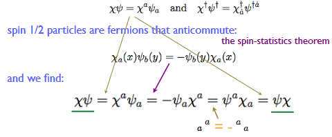
snippet grabbed from (Dermisek 09)
We analyze the special nature of the supergeometry space of field histories of the Dirac field a little (prop. 3.51) below and conclude by highlighting the crucial role of supergeometry (remark 3.52 below)
Proposition 3.51. (space of field histories of the Dirac field)
Let ##E = \Sigma \times S_{odd} \overset{pr_1}{\to} \Sigma## be the super-field bundle (def. 3.45) for the Dirac field over Minkowski spacetime ##\Sigma = \mathbb{R}^{p,1}## from example 3.50.
Then the corresponding supergeometric space of field histories
$$
\Gamma_\Sigma(\Sigma \times S_{odd})
\;\in\;
SuperSmoothSet
$$
from example 3.46 has the following properties:
- For ##U = \mathbb{R}^n## an ordinary Cartesian space (with no super-geometric thickening, def. 3.37) there is only a single ##U##-parameterized collection of field histories, hence a single plot$$
\Psi_{(-)}\;\colon\;\mathbb{R}^n \overset{ 0 }{\longrightarrow} \Gamma_\Sigma(\Sigma \times S_{odd})
$$and this corresponds to the zero section, hence to the trivial Dirac field$$
\Psi^A_{(-)} = 0
\,.
$$ - For ##U = \mathbb{R}^{n \vert 1}## a super Cartesian space (3.37) with a single super-odd dimension, then ##U##-parameterized collections of field histories$$
\Psi_{(-)} \;\colon\; \mathbb{R}^{n\vert 1} \longrightarrow \Gamma_\Sigma(\Sigma \times S_{odd})
$$are in natural bijection with plots of sections of the bosonic-field bundle with field fiber ##S_{even} = S## the spin representation regarded as an ordinary vector space:$$
\theta \Psi_{(-)} \;\colon\; \mathbb{R}^n \longrightarrow \Gamma_\Sigma(\Sigma \times S_{even})
\,,
$$
Moreover, these two kinds of plots determine the fermionic field space completely: It is in fact isomorphic, as a super vector space, to the bosonic field space shifted to odd degree (as in example 3.38):
$$
\Gamma_\Sigma(\Sigma \times S_{odd})
\;\simeq\;
\left(
\Gamma_\Sigma(E\times S_{even})
\right)_{odd}
\,.
$$
Proof. In the first case, the plot is a morphism of super Cartesian spaces (def. 3.37) of the form
$$
\mathbb{R}^n \times \mathbb{R}^{p,1} \longrightarrow S_{odd}
\,.
$$
By definitions, this is dually homomorphism of real supercommutative superalgebras
$$
C^\infty(\mathbb{R}^n \times \mathbb{R}^{p,1}) \longleftarrow \wedge^\bullet S^\ast
$$
from the Grassmann algebra on the
For the second case, notice that a morphism of the form
$$
\mathbb{R}^{n\vert 1}
\overset{\Psi_{(-)}}{\longrightarrow}
S_{odd}
$$
is by def. 3.48 naturally identified with a morphism of the form
$$
\mathbb{R}^n \overset{}{\longrightarrow} [\mathbb{R}^{0 \vert 1}, S_{odd}] \simeq S_{odd} \times S_{even}
\,,
$$
where the identification on the right is from example 3.49.
By the nature of Cartesian products, these morphisms, in turn, are naturally identified with pairs of morphisms of the form
$$
\left(
\array{
\mathbb{R}^n &\overset{}{\longrightarrow}& S_{odd}\,,
\\
\mathbb{R}^n &\overset{}{\longrightarrow}& S_{even}
}
\right)
\,.
$$
Now, as in the first point above, here, the first component is uniquely fixed to be the zero morphism ##\mathbb{R}^n \overset{0}{\to} S_{odd}##, and hence only the second component is free to choose. This is precisely the claim to be shown.
Remark 3.52. (supergeometric nature of the Dirac field)
Proposition 3.51 how two basic facts about the Dirac field, which may superficially seem to be in tension with each other, are properly unified by supergeometry:
- On the one hand, a field history ##\Psi## of the Dirac field is not an ordinary section of an ordinary vector bundle. In particular, its component functions ##\psi^A## anti-commute with each other, which is not the case for ordinary functions, and this is crucial for the Lagrangian density of the Dirac field to be well defined, we come to this below in example 5.8.
- On the other hand, a field history of the Dirac field is supposed to be a spinor, hence a section of a spinor bundle, which is an ordinary vector bundle.
Therefore prop. 3.51 serves to shows how, even though a Dirac field is not defined to be an ordinary section of an ordinary vector bundle, it is nevertheless encoded by such an ordinary section: One says that this ordinary section is a “superfield-component” of the Dirac field, the one linear in a Grassmann variable ##\theta##.
This concludes our discussion of the concept of fields itself. In the following chapter we consider the variational calculus of fields.
I am a researcher in the department Algebra, Geometry and Mathematical Physics of the Institute of Mathematics at the Czech Academy of the Sciences (CAS) in Prague.
Presently I am on leave at the Max Planck Institute for Mathematics in Bonn.


But the notion of positivity is questionable in algebras over rings of formal power series since the latter have no total linear order.It's formal power series algebras equipped with star-algebra structure and positivity is defined in terms of the star algebra structure.
Right, one uses the positivity of a given state (one of the axioms on a state on an algebra of observables).In the quoted Nlab article you write (and implicitly you usie this in the present discussion, too):
the definition [of a state] makes sense generally for plain star-algebras, such as for instance for the formal power series algebras that appear in perturbative quantum field theoryBut the notion of positivity is questionable in algebras over rings of formal power series since the latter have no total linear order. Using a partial order instead provides some notion of positivity but not the physical one.In the physical setting, ##hbar_{phys}-hbar_{formal}ge 0##, while in the formal setting, this is not the case.
In the equilibrium case you also have a kind of "adiabatic switching" by pushing the initial time to ##-infty## to get rid in a subtle way of the necessity to consider the vertical pieces in the extended Schwinger-Keldysh contour. This is another often discussed subtlety in the real-time community. In my opinion it's completely settled in F. Gelis's papers, where it is shown that in fact you can take the initial time finite (but "earlier" than any time argument in the to be evaluted Green's functions), as to be expected from the fact that one deals with equilibrium which is by definition stationary and thus time-translation invariant. From another point of view, it's only important to keep track of the correct "causal regularization" of the on-shell ##delta## distributions in the free Schwinger-Keldysh-contour propgators, used in perturbation theory.
F. Gelis, The Effect of the vertical part of the path on the real time Feynman rules in finite temperature field theory, Z. Phys. C, 70 (1996), p. 321–331.
http://dx.doi.org/10.1007/s002880050109
F. Gelis, A new approach for the vertical part of the contour in thermal field theories, Phys. Lett. B, 455 (1999), p. 205–212.
http://dx.doi.org/10.1016/S0370-2693(99)00460-8
Well, ##hbar## is still a number, which is empirically defined. In fact it's a unit-conversion factor and I'm pretty sure that it will be defined officially next year to update the SI for the 21st century and to take legal effect in 2019.But in the theoretical exposition of Urs Schreiber (and implicitly in perturbative QFT in general) it is a parameter in a power series with zero convergence radius. Thus inserting a finite positive value gives results depending on the order of calculation, and diverging if the order is taken too high. Haag and Kastler, to whom he had referred, were using true operators, not formal power series operators.
The considered quantities at "finite times" ("transient states") are off by orders of magnitude and, as far as we could figure out, don't have a clear physical interpretation but are calculational tools only.Well, at least in the equilibrium case (and in fact more generally in the hydrodynamic limit), they have a very tangible measurable meaning at finite times.
And one has to give up the idea that ##hbar## is a number – instead it is only a formal parameter! And one has to give up the idea that operators act on more than a compact part of space-time – to avoid all the infrared problems.Well, ##hbar## is still a number, which is empirically defined. In fact it's a unit-conversion factor and I'm pretty sure that it will be defined officially next year to update the SI for the 21st century and to take legal effect in 2019.
How can you say that? In your work you don't only discuss S-matrix elements but all the correlation functions, related by Kadanoff-Baym equations!Yes, but at the end we use these correlation functions to measure spectra of "particles", and these are defined as asymptotic free space. Of course, we do this in the naive mathematically non-rigorous way, using the usual recipies like adiabatic switching and all that. Our conclusion at the time of writing these articles (see, particularly the Annals of Physics one) that one has to do the good old Gell-Mann-Low switching for both "switching on and off the interactions" to make pysical sense of the photon spectra. The considered quantities at "finite times" ("transient states") are off by orders of magnitude and, as far as we could figure out, don't have a clear physical interpretation but are calculational tools only.
The point of "perturbative AQFT" is to notice that if one keeps everything about Haag-Kastler except the demand that the star-algebras of observables have a ##C^*##-algebra structure,And one has to give up the idea that ##hbar## is a number – instead it is only a formal parameter! And one has to give up the idea that operators act on more than a compact part of space-time – to avoid all the infrared problems.
Well, the physical interpretation of Heisenberg field operators is highly non-trivial, if not even one can say it basically doesn't exist. That's the reason why one finally only discusses S-matrix elementsHow can you say that? In your work you don't only discuss S-matrix elements but all the correlation functions, related by Kadanoff-Baym equations!
Clearly the old Schwinger-Tomonaga-Feynman-Dyson renormalization is to be disliked. But I think this is unrelated to the issue of the Schrödinger picture that I just mentioned. Essentially nobody ever works or worked in the Schrödinger picture in QFT, it's only that people fall back to it when trying to conceptualize what they are doingWell, there's one book, treating the Schrödinger picture in relativistic QFT (although I never understood, why I should use it for this purpose anyway):
B. Hatfield, Quantum Field Theory of Point Particles and Strings, Addison-Wesley, Reading, Massachusetts, 10 ed., 1992.
in the Heisenberg picture the Hilbert space of states is secondary. What is primary is the algebra of observables together with one state on them (the vacuum or ground state). Of course, as Arnold recalled above, under good circumstances a Hilbert space of states may be reconstructed from this data, but this is usually an afterthought, not key for the core computations.The GNS construction always associates to the vacuum state a Hilbert space representing the algebra. The only requirement is that the vacuum state is a positive linear functional of the associated *-algebra; this basic property is a necessary physical requirement. Thus the Hilbert space is as relevant to the Heisenberg picture as it is to the Schrödinger picture. The only difference is that the Heisenberg picture is manifestly covariant, while the Schroedinger picture assumes a preferred frame (or foliation) .
Note that perturbative QFT neither constructs the observable algebra nor a positive vacuum state. (Constructing both would imply having constructed a model of the Wightman axioms.) Instead it constructs an approximate algebra in a Fock space corresponding to an asymptotic state space. This asymptotic subspace is unphysical, as it treats both infraparticles such as the electron and confined quarks as asymptotic particles. This is the deeper origin of the infrared problems.
Thus taking the Hilbert space as only an afterthought of QFT is one of the roots of the main unsolved problems in the area.
Yes, that's what "enters". But section 8 doesn't derive the quantum angular momentum spectrum. The output is important here, not just what "enters". The closest it gets is a passing mention of an eigenvalue equation for ##L^2## in terms of ordinary wave functions.
"Most" being the key word here. The point of my challenge to try and establish whether derivation of the quantum angular momentum spectrum is one of the cases in QM for which a Hilbert space is essential.
You're not the first person to whom I have offered this challenge. But so far, no one has actually provided a satisfactory response (nor reference) to the point of the challenge, instead evading that point by giving references that don't actually address the point, and (eventually) by unhelpful denigration of other authors. I grow concerned that you seem to be sliding into the latter category.
I also notice that you ignored my question about whether you have a copy of Ballentine there to refer to. I guess your non-response means "no"?I don't understand what's the issue with angular momentum. It's a nice operator algebra of a compact semisimple Lie algebra and as such doesn't make any trouble at all in the standard Hilbert-space theory. You construct them algebraically via raising- and lowering operators or, even more convenient, using the fact that the 2D harmonic oscillator has SU(2) symmetry and construct everything with annihilation and creation phonon operators.
For orbital angular momentum you also get a very elegant derivation of the spherical harmonics by just writing the algebraic findings in position representation. I think it's very easy to make this also mathematically rigorous in the standard Hilbert-space representation. It's of course the same in relativistic and non-relativistic physics, because SO(3) is a subgroup of both the proper orthochronous Poincare as well as the Galileo group.
In other words: What do you use instead of the standard Hilbert space concept to define states (represented by statistical operators, where pure states are special cases being represented by projection operators) and why should one do so?
Here I am not fully certain what this is arguing about. If you mean Heisenberg picture as opposed to interaction picture, hence non-perturbative as opposed to perrturbative, then there is a dearth of examples, sure, but no conceptual issue.It's about physics. You have no particle interpretation of transient states. For practical purposes, it's a delicate issue. One example is the off-equilibrium production of photons in heavy-ion collisions. There was quite some debate due to these problems. We have investigated it for a simple toy model (photon production due to a time-dependent scalar background field):
F. Michler, H. van Hees, D. D. Dietrich, C. Greiner, Asymptotic description of finite lifetime effects on the photon emission from a quark-gluon plasma
Phys. Rev. D 89, 116018 (2014)
arXiv: 1310.5019 [hep-ph]
F. Michler, H. van Hees, D. D. Dietrich, S. Leupold, C. Greiner, Off-equilibrium photon production during the chiral phase transition
Contribution to the proceedings of the 51st International Winter Meeting on Nuclear Physics, 21-25 January 2013, Bormio (Italy)
PoS Bormio2013, 055 (2013)
arXiv: 1304.4093 [nucl-th]
F. Michler, H. van Hees, D. D. Dietrich, S. Leupold, C. Greiner, Non-equilibrium photon production arising from the chiral mass shift
Ann. Phys. 336, 331 (2013)
arXiv: 1208.6565 [nucl-th]
It's not about the mathematics, and I'm quite sure that the formalism gets the standard perturbation theory right, but it's about the physics interpretation, and there also the axiomatic approach deals with ther properly defined in physically interpretable S-matrix elements, i.e., the transition amplitudes from asymptotic free in to asymptotic free out states. Only the asymptotic free states have a clear particle interpretation, not any quantities in "transient states".
Section 8 that the discussion relies on is aptly titled "Commutation relations". That means: The algebra structure of the algebra of observables. That's what enters. Yes, that's what "enters". But section 8 doesn't derive the quantum angular momentum spectrum. The output is important here, not just what "enters". The closest it gets is a passing mention of an eigenvalue equation for ##L^2## in terms of ordinary wave functions.
You can tell that most constructions in quantum mechanics don't necessarily need the Hilbert space concept […] "Most" being the key word here. The point of my challenge to try and establish whether derivation of the quantum angular momentum spectrum is one of the cases in QM for which a Hilbert space is essential.
You're not the first person to whom I have offered this challenge. But so far, no one has actually provided a satisfactory response (nor reference) to the point of the challenge, instead evading that point by giving references that don't actually address the point, and (eventually) by unhelpful denigration of other authors. I grow concerned that you seem to be sliding into the latter category.
I also notice that you ignored my question about whether you have a copy of Ballentine there to refer to. I guess your non-response means "no"?
the physical interpretation of Heisenberg field operators is highly non-trivialHere I am not fully certain what this is arguing about. If you mean Heisenberg picture as opposed to interaction picture, hence non-perturbative as opposed to perrturbative, then there is a dearth of examples, sure, but no conceptual issue. On the contrary, the Haag-Kastler AQFT axtioms are all about this: axiomatizing the Heisenberg picture observables in QFT, and that's just where the algebraic definition of quantum state that I have been highlighting originates. The point of "perturbative AQFT" is to notice that if one keeps everything about Haag-Kastler except the demand that the star-algebras of observables have ##C^ast##-algebra structure, then one gets a precise conceptualization of traditional perturbative quantum field theory.
So the trick is that you only need the vacuum state and then reconstruct everything through the N-point functions, defined as "vacuum expectation values"? That's very interesting since it sounds intuitively to be sufficient to define S-matrix elements for definite scattering processes since for asymptotic free states you have a particle interpretation.I would say that's just how pQFT works: We fix a vacuum state, given by a linear map
$$langle -rangle ;:; mathrm{NiceEnoughObservables} longrightarrow mathbb{C}$$
(on curved spacetimes a Hadamard state) and then for incoming field excitations at ##x_{in,i}## in state ##a_{in,i}## and outgoing field excitations at ##x_{out,j}## in state ##b_{out,j}## we form the observable
$$ left( mathbf{Phi}^{a_{out,1}}(x_{out,1}) cdots mathbf{Phi}^{a_{out,n_{out}}}(x_{in,n_{out}}) right)^ast , S_g , mathbf{Phi}^{a_{in,1}}(x_{in,1}) cdots mathbf{Phi}^{a_{in,n_{in}}}(x_{in,n_{in}}) ;in; mathrm{Observables} $$
and then apply the above vacuum state to it to produce a function (in fact a generalized function) in the positions ##x##
$$leftlangle left( mathbf{Phi}^{a_{out,1}}(x_{out,1}) cdots mathbf{Phi}^{a_{out,n_{out}}}(x_{in,n_{out}}) right)^ast , S_g , mathbf{Phi}^{a_{in,1}}(x_{in,1}) cdots mathbf{Phi}^{a_{in,n_{in}}}(x_{in,n_{in}}) rightrangle $$
If we are attached to the idea of Hilbert spaces, then we write this as
$$ leftlangle mathbf{Phi}^{a_{out,1}}(x_{out,1}) cdots mathbf{Phi}^{a_{out,n_{out}}}(x_{in,n_{in}}) rightvert , S_g , leftvert mathbf{Phi}^{a_{in,1}}(x_{in,1}) cdots mathbf{Phi}^{a_{in,n_{in}}}(x_{in,n_{in}}) rightrangle $$
and feel that we have justified the term "matrix" in "S-matrix". But the previous notation is better for reminding us that all we actually need to use is a single state: the vaccuum state (generally: Hadamard state).
Dirac always disliked re-normalization.Clearly the old Schwinger-Tomonaga-Feynman-Dyson renormalization is to be disliked. But I think this is unrelated to the issue of the Schrödinger picture that I just mentioned. Essentially nobody ever works or worked in the Schrödinger picture in QFT, it's only that people fall back to it when trying to conceptualize what they are doing
No, this applies generally, also to interacting theory. In pQFT what changes as one turns on the interaction is that the Wick normal ordred product on observables gets deformed into the "retarded products" (the infinitesimal version of Bogoliubov's formula) and then it's still the vacum state (or more generally Hadamard state) which serves to send such products of observables to their actual expectation value, which is the corresponding correlator.Well, the physical interpretation of Heisenberg field operators is highly non-trivial, if not even one can say it basically doesn't exist. That's the reason why one finally only discusses S-matrix elements, which rely on asymptotic free in and out states which have a proper particle interpretation. To make sense of transit states is usually not even considered!
Absolutely. And in the Schrödinger picture a Hilbert space of states needs to be assumed from the outset, while in the Heisenberg picture it is an afterthought, if it exsists at all. What matters in the Heisenberg picture is that we know one state, the vacuum state, given as a positive linear non-degenerate function which sends observables to their expectation value. In optimal situation the GNS construction allows to reconstruct a Hilbert space from this, but not generally (notably not in interacting pQFT).
And that's where it begins to be misleading. First of all the representation of observables as operators on a Fock space is not necessary for the construction of the Wick algebra and second it does not generally exist for QFT on curved backgrounds. Instead what one needs is the Hadamard propagator which allows to construct the Wick algebra of observables and at the same time defines a single state (positive linear non-degenrate functional on observables) on this.So the trick is that you only need the vacuum state and then reconstruct everything through the N-point functions, defined as "vacuum expectation values"? That's very interesting since it sounds intuitively to be sufficient to define S-matrix elements for definite scattering processes since for asymptotic free states you have a particle interpretation.
The Fock space is a Hilbert space, yes. In good cases it happens to exist. In general it does not, and even if it does, it is not actually necessary to do any and all of pQFT.”
On the one hand there are intrinsic problems with applying the Hilbert space Schrödinger picture to QFT even in principle (Torre-Varadarajan 98).Dirac always disliked re-normalization. But I did read somewhere by using the Heisenberg picture he did obtain the same results without it. Evidently they were long but it did work.
Thanks
Bill
Whats your view of resolving it with Rigged Hilbert Spaces and the Generalized Spectral Theorem?These are good tools if one wants to be serious about Schrödinger-picture quantum mechanics.
There is good stuff to be found in the Hilbert space Schrödinger picture, if done with due care (as amplified in texts like "Self-adjoint extensions of operators and the teaching of quantum mechanics").
One just has to exercise care with regarding this good QM stuff as indication that the Schrödinger picture is a robust foundation for quantum physics in a generality that includes QFT. It turns out that it is not. On the one hand there are intrinsic problems with applying the Hilbert space Schrödinger picture to QFT even in principle (Torre-Varadarajan 98). On the other hand the Heisenberg/interaction picture without a choice of Hilbert space (just with the option to find one, if possible) works wonders and is in fact, more or less secretly, precisely what everyone uses in practice anyway, even if it superficially seems as if Hilbert spaces are being used.
There are issues of dense sub-domains of unbounded operators, of self-adjoint extensions of symmetric operators on a Hilbert space etc. that need to be dscussed if one is really speaking Hilbert spaces.Too true.
Whats your view of resolving it with Rigged Hilbert Spaces and the Generalized Spectral Theorem?
Thanks
Bill
Well, I guess that refers to free particlesNo, this applies generally, also to interacting theory. In pQFT what changes as one turns on the interaction is that the Wick normal ordred product on observables gets deformed into the "retarded products" (the infinitesimal version of Bogoliubov's formula) and then it's still the vacum state (or more generally Hadamard state) which serves to send such products of observables to their actual expectation value, which is the corresponding correlator.
in the Heisenberg picture (which is anyway the most natural picture to use; it's only due to overemphasizing wave mechanics rather than the canonical approach, why in QM 1 we usually start with the Schroedinger picture).Absolutely. And in the Schrödinger picture a Hilbert space of states needs to be assumed from the outset, while in the Heisenberg picture it is an afterthought, if it exsists at all. What matters in the Heisenberg picture is that we know one state, the vacuum state, given as a positive linear non-degenerate function which sends observables to their expectation value. In optimal situation the GNS construction allows to reconstruct a Hilbert space from this, but not generally (notably not in interacting pQFT).
Then we construct the Fock space as the occupation-number eigenstates (usually in the single-particle momentum representation).And that's where it begins to be misleading. First of all the representation of observables as operators on a Fock space is not necessary for the construction of the Wick algebra and second it does not generally exist for QFT on curved backgrounds. Instead what one needs is the Hadamard propagator which allows to construct the Wick algebra of observables and at the same time defines a single state (positive linear non-degenrate functional on observables) on this.
Now, isn't his a Hilbert spaceThe Fock space is a Hilbert space, yes. In good cases it happens to exist. In general it does not, and even if it does, it is not actually necessary to do any and all of pQFT.
Then he uses positivity of the Hilbert space inner productRight, one uses the positivity of a given state (one of the axioms on a state on an algebra of observables).
Nanni's section 12 (wherein he searches for a suitable factorization of the Hamiltonian) relies on results back in sections 6,7,8 concerning angular momentumSection 8 that the discussion relies on is aptly titled "Commutation relations". That means: The algebra structure of the algebra of observables. That's what enters.
You can tell that most constructions in quantum mechanics don't necessarily need the Hilbert space concept by the simple fact that most standard textbooks and most students don't even know the functional analysis involved when really considering Hilbert spaces, and not just commutation relations. There are issues of dense sub-domains of unbounded operators, of self-adjoint extensions of symmetric operators on a Hilbert space etc. that need to be discussed if one is really speaking Hilbert spaces. The reason that students and textbooks get away without even mentioning this (such as Ballentine's book) is due to the fact that from just the algebra structure (commutators) of the observables and the basic properties of states (linearity, normalization, positivity) as functions from observables to complex numbers, one can obtain most results.
But you are secretly very familiar with this Heisenberg-picture perspective, because this is precisely what traditional perturbative QFT is based on. There we have the ##n##-point functions or scattering amplitudes defined as linear functionals on the collection of products of field observables, with respect to a "vacuum state" which is implicitly defined thereby, and no Hilbert space needs to be mentioned to speak about these. In fact for pQFT in curved spacetime no such Hilbert space needs to exist, and still the standard machine applies.Well, I guess that refers to free particles in the Heisenberg picture (which is anyway the most natural picture to use; it's only due to overemphasizing wave mechanics rather than the canonical approach, why in QM 1 we usually start with the Schroedinger picture). Then we construct the Fock space as the occupation-number eigenstates (usually in the single-particle momentum representation). Now, isn't his a Hilbert space (at least for a finite quantization volume imposing periodic boundary conditions)? I'll have a look at the mentioned lecture notes by Fredenhagen et al.
You'll notice that what this computation (in Ballentine or elsewhere) really uses is the commutation relations of the angular momentum observables together with one ground state they act on. Well,… no, I don't notice that. (Do you have a copy of Ballentine in front of you?)
I see (on p160) that he starts by recognizing ##J^2## and ##J_z## as commuting self-adjoint operators. Hence if they act on a Hilbert space, that Hilbert space is spanned by common eigenvectors parameterized by the eigenvalues of these operators (##beta,m##). Then he uses positivity of the Hilbert space inner product to derive an inequality ##beta ge m^2## in eq(7.4). Then he use the ladder operators ##J_pm## and the inequality (7.4) to show that repeated application of either ladder operator eventually gives 0, and for any given value of ##beta## there is a maximum value "##j##" of ##m##. Thus he deduces the dimension of the Hilbert space for any given value of ##beta##, and also that ##beta = j(j+1)## — eq(7.10).
For amplification see for instance also the quantization of the hydrogen atom in the Heisenberg picture, e.g. section 12 of Nanni 15. Nanni's section 12 (wherein he searches for a suitable factorization of the Hamiltonian) relies on results back in sections 6,7,8 concerning angular momentum properties of wave functions found from the usual Schrodinger equation.
Well, then I've big trouble making any sense of QFT at all since then I don't know, how to define states and how to interpret the S-matrix physically, or how do you define states and probabilities in a theory without an underlying Hilbert space.This is the old concept of state in AQFT, I recommend the lecture notes Fredenhagen 03 (section 2) for the non-perturbative (##C^ast##-algebraic) version and Fredenhagen-Rejzner 12 (around def. 2.4) as well as Rejzner 16 (starting with section 2.1.2) for the perturbative QFT version (just dropping the ##C^ast##-condition).
But you are secretly very familiar with this Heisenberg-picture perspective, because this is precisely what traditional perturbative QFT is baseThed on. There we have the ##n##-point functions or scattering amplitudes defined as linear functionals on the collection of products of field operators, with respect to a "vacuum state" which is implicitly defined thereby, and no Hilbert space needs to be mentioned to speak about these. In fact for pQFT in curved spacetime no such Hilbert space needs to exist, and still the standard machine applies.
We will come to this in the series in chapters 14. Free quantum fields and 16. Quantum observables.
Regarding Epstein-Glaser 73, what they achieved is to axiomatiize the properties of the perturbative S-matrix, thereby making sense of the would-be path integral, and proving that from these (very simple) axioms the construction of pQFT via renormalization by splitting/extension of the distributions given by the Feynman diagrams (here). Hence they managed to make good sense of (Lorentzian) pQFT.
We come to this in the series in chapter 15. Scattering.
Well, then I've big trouble making any sense of QFT at all since then I don't know, how to define states and how to interpret the S-matrix physically, or how do you define states and probabilities in a theory without an underlying Hilbert space. Of course, the general state is uniquely represented by a Statistical Operator rather than a Hilbert-space vector (or ray), but to make sense of the Statistical Operator you need at least a trace operation. Can this be defined without relying on a Hilbert-space concept?
I always thought the success of perturbative QFT, despite being mathematically quite undefined, is that the physicists intuitively take the limits in their calculations in a correct way, even although they are not able to rigorously define them in a mathematically satisfactory strict sense. Of course, I have in mind things like using a finite quantization volume (with periodic boundary conditions), adiabatic switching a la Gell-Mann and Low and various regularization procedures for divergent perturbative integrals (loops and Feynman diagrams), or appropriate counterterm-subtraction techniques without regularization (a la BPHZ) to make sense of the ill-defined divergent integrals.
I thought, particularly the Epstein-Glaser causal approach, is just another particularly physical way to take these limits in using "smeared" field operators, which makes a lot of physical sense, particularly in view of the Wilson approach to renormalization and his physical interpretation of the renormalization-group equations, and I also thought that this is at least some step towards a mathematically more satisfying foundation in providing the correct rules of mutliplying distribution-like operators or Green's and vertex functions.
derive the usual quantum angular momentum spectrum without using a Hilbert space (directly or indirectly). Cf. Ballentine section 7.1 where he derives that spectrum from little more than the requirement to represent SO(3) unitarily on an abstract Hilbert space. :oldbiggrin:You'll notice that what this computation (in Ballentine or elsewhere) really uses is the commutation relations of the angular momentum observables together with one ground state they act on. For amplification see for instance also the quantization of the hydrogen atom in the Heisenberg picture, e.g. section 12 of Nanni 15.
In passing from quantum mechanics to quantum field theory, it is important to notice that it is the Heisenberg picture (or interaction picture for perturbation theory) that generalizes well, not the Schrödinger picture (see also Torre-Varadarajan 98 for issues with the Schrödinger picture in QFT). Those quantum field observables ##mathbf{Psi}(x)## that we have been discussing elsewhere, they are the hallmark of the Heisenberg picture. And in th Heisenberg picture the Hilbert space of states is secondary. What is primary is the algebra of observables together with one state on them (the vacuum or ground state). Of course, as Arnold recalled above, under good circumstances a Hilbert space of states may be reconstructed from this data, but this is usally an afterthought, not key for the core computations.
If one looks at old articles such as the original Epstein-Glaser article on causal perturbation theory, they always carry around phrases like "assuming that all operators involved can be chosen to have joint dense domain of definition" etc., which comes from insisting that the quantum observables be represented on a Hilbert space. But in fact this is an unnecessary asumption for the results of causal perturbation theory, everything goes through directly with considering just the "abstract" algebra of observables. It's easier, less conceptual baggage.
That is not to say that having a Hilbert space representation is not useful. But its not conceptually primary for the development of QFT.
perhaps you could insert something like the last part of this sentence near the place where you define "field history"?Good point. Will do.
The QFT textbook to recommend, as I did before, which gets the concepts right, is
Amazon has one copy left – may snap it up as a Christmas gift.
But it occurs to me, and this is something I have been meaning to investigate for some time now, it looks related to the latter work of Von-Neumann on C*algebras and QM. Would that be correct?. Of course I have read his classic Mathematical Foundations which is done entirely in Hilbert Spaces. In fact it was one of the first proper books on QM I ever read. Having studied Hilbert spaces as part of my degree it was a piece of cake so to speak – the other one I read – Dirac – was a big problem and I had to investigate RHS's to finally get a grip on it. When I did it was the other way around – I preferred Dirac to Von-Neumann.
Would the following be a good primer for the book you mentioned, as well as your whole series?
http://www.math.uchicago.edu/~may/VIGRE/VIGRE2009/REUPapers/Gleason.pdf
It has more formal math than I am used to these days – like Varadarajan it looks a bit of a 'slog' but if valuable will persevere.
Thanks
Bill
Why the change from "configuration" to "history"?Because it's more appropriate in the Lorentzian setup, where a section of the field bundle is a field configuration over every spatial slice together with its change in time, hence a history. OK, that's fine. But perhaps you could insert something like the last part of this sentence near the place where you define "field history"?
When looking closely at field theory, it turns out that this is unhelpful, that other concepts are prior, and that a Hilbert space of states is an addendum to be considered after the theory has been constructed algebraically. States are a priori positive linear functionals on the abstractly defined algebra of quantum observables, and representing the latter on a Hilbert space may be a convenient tool for ensuring positivity of such functionals, but it is neither necessary nor in general possible or helpful. Well, then I respectfully challenge you to derive the usual quantum angular momentum spectrum without using a Hilbert space (directly or indirectly). Cf. Ballentine section 7.1 where he derives that spectrum from little more than the requirement to represent SO(3) unitarily on an abstract Hilbert space. :oldbiggrin:
epresenting the latter on a Hilbert space may be a convenient tool for ensuring positivity of such functionals, but it is neither necessary nor in general possible or helpful.This may be the current state of the art in 4D relativistic quantum theory, but this is only because we still lack the right mathematical tools. A nonperturbative mathematical construction of any QFT will necessarily produce a representation of the (bounded part of the) quantum algebra on a Hilbert space of physical states. Each positive linear functional provides such a Hilbert space, and inequivalent representations are accounted for by taking a direct sum.
Besides the condition of gauge invariance on observables that you mention, there are various further conditions which need to be considered. In the end the quantum algebra is based only on those observables which in addition are also local and microcausal. Also "on-shell" will have to be added as a qualifier, since it is useful also to consider off-shell observables.
For this reason, it is natural to say just "observable" for any functional on the space of field histories, and then eventually to add adjectives as one specializes. Citing from the lead-in paragraphs of chapter 7:
There are various further conditions on observables which we will eventually consider, forming subspaces of gauge invariant observables (def. 11.2), local observables (def. 7.35 below), Hamiltonian local observables (def. 8.12 below) and microcausal observables (def. 14.5). While in the end it is only these special kinds of observables that matter, it is useful to first consider the unconstrained concept and then consecutively characterize smaller subspaces of well-behaved observables. In fact it is useful to consider yet more generally the observables on the full space of field histories (not just the on-shell subspace), called the off-shell observables.I'm not so much concerned about the use of the term "observable". That's anyway finally defined as something that's indeed measured in the lab, and the (far from trivial!) task of any quantum-field theory is to map the formalism to this operational definition of "observable". I'm a bit quibbled, why you use the term "field histories". A "history", as I understand the term, is a sequence of observed facts, but as we seem to agree upon, the fundamental fields are usually not directly observables in the formalism but are used to construct observables (or more carefully stated the corresponding representing operators of observables) via a local realization of the Poincare algebra.
Another trouble is caused by taking the infinite-volume limit. Haag's theorem is related to it. See, e.g.,
A. Duncan, The conceptual framework of QFT, Oxford University Press (2012) Sect. 10.5
I'd propose to use ''quantity'' for any functional on the space of field historiesThat seems overly unspecific and also unconventional
It is completely conventional and useful to speak of "local gauge-invariant on-shell observables" and we couldn't do that if we defined "observanle" to already mean "local gauge invariant on-shell observables".
To relativize concern about the choice of terminology remember that even with plenty of qualifiers added, the mathematical concept of "observable" is necessarily still a highly idealized formalization of what happens to our sensory system as we make an observation in nature (for one we haven't even touched general covariance yet, or noise or coarse graining, not to speak of biological and psychological aspects), so it seems misguided to be pedantic about naturalistic linguistic here over having a useful crisp technical terminology.
I am sure you have read, as have I, the following:
https://www.amazon.com/Geometry-Quantum-Theory-V-S-Varadarajan/dp/0387493859
I don't know if you have read Ballentine:
https://www.amazon.com/Quantum-Mechanics-Modern-Development-2nd/dp/9814578576
A number on this forum, me included, tend to think of Ballentine as our bible on QM.Ballentine's book as well as Varadarajan's both having emphasis on QM over QFT, put the concept of a Hilbert space of states in the center of attention. When looking closely at field theory, it turns out that this is unhelpful, that other concepts are prior, and that a Hilbert space of states is an addendum to be considered after the theory has been constructed algebraically. States are a priori positive linear functionals on the abstractly defined algebra of quantum observables, and representing the latter on a Hilbert space may be a convenient tool for ensuring positivity of such functionals, but it is neither necessary nor in general possible or helpful. We'll get to that in the series in chapters 14 and 16.
The QFT textbook to recommend, as I did before, which gets the concepts right, is
There are various further conditions on observables which we will eventually consider, forming subspaces of gauge invariant observables (def. 11.2), local observables (def. 7.35 below), Hamiltonian local observables (def. 8.12 below) and microcausal observables (def. 14.5). While in the end it is only these special kinds of observables that matter, it is useful to first consider the unconstrained concept and then consecutively characterize smaller subspaces of well-behaved observables. In fact it is useful to consider yet more generally the observables on the full space of field histories (not just the on-shell subspace), called the off-shell observables.I'd propose to use ''quantity'' for any functional on the space of field histories, and ''observable'' for those quantities that are actually observable.
But as to why it happensAllow me to suggest that it (namely the suggestion that researchers sit in camps that constrain their ability to think about the total nature of the problem at hand) happens out of intellectual laziness. It takes little effort to copy quotes from Wikipedia that make fun of people in what is perceived a different camp, while it takes effort to learn all aspects of the problem and transcend the camp spirit.
I think it is plain obvious that to understan QFT you need all of it: A good idea of its physical meaning as well as the mathematical tools that it takes not to get confused (say about what "field" means in field theory…)
but the choice of words, which may mislead a beginner to think that the fundamental field operators are observables.Besides the condition of gauge invariance on observables that you mention, there are various further conditions which need to be considered. In the end the quantum algebra is based only on those observables which in addition are also local and microcausal. Also "on-shell" will have to be added as a qualifier, since it is useful also to consider off-shell observables.
For this reason, it is natural to say just "observable" for any functional on the space of field histories, and then eventually to add adjectives as one specializes. Citing from the lead-in paragraphs of chapter 7:
There are various further conditions on observables which we will eventually consider, forming subspaces of gauge invariant observables (def. 11.2), local observables (def. 7.35 below), Hamiltonian local observables (def. 8.12 below) and microcausal observables (def. 14.5). While in the end it is only these special kinds of observables that matter, it is useful to first consider the unconstrained concept and then consecutively characterize smaller subspaces of well-behaved observables. In fact it is useful to consider yet more generally the observables on the full space of field histories (not just the on-shell subspace), called the off-shell observables.
In "aspects of the concept of fields" appears the notation ##delta_{EL}=0##. Later, under Remark 3.2. (possible field histories), it reappears as ##delta_{EL}{mathbf L}=0##. Is that a typo?That's a typo, yes. I am fixing it.
Why the change from "configuration" to "history"?Because it's more appropriate in the Lorentzian setup, where a section of the field bundle is a field configuration over every spatial slice together with its change in time, hence a history.
And why not call it simply "field on spacetime"?Because this is too ambiguous and leads to confusion. For instance when we say "consider the electromagnetic field" we are not referring to a specific field history, but to the type of possible field histories.
I guess that's to make a distinction between smooth/rough fields?No.
But do we ever need rough fields in QFT?If you mean non-smooth field histories, then: No.
Most of the fundamental fields in the standard model are not representing observables directly:Got it :biggrin::biggrin::biggrin::biggrin::biggrin:
Thanks
Bill
In fact many seem to think that taking that blob size to zero is the cause of much of the issues in QFT.In nonrelativistic QFT this causes no problems. The problems are intrinsically relativistic – in preserving Poincare invariance.
I'm going back and re-reading some stuff. In the "Fields" installment, you (@Urs Schreiber) say: However, the nLab entry says: Why the change from "configuration" to "history"?
And why not call it simply "field on spacetime"? I guess that's to make a distinction between smooth/rough fields? But do we ever need rough fields in QFT?Indeed, using the term "field configuration" makes it much better!
When one quantizises a quantum field at an intuitive level its the same as what's going on with a classical field as you would find in a book on classical field theory such as the one I have by Soper – Classical Field Theory. What you do is think of the field as a lot of small blobs interacting in some way. When it's quantisized the properties of those small blobs – whatever they are – momentum, position, electric field strength, or whatever are quanatizised and become operators. Then the blob size is taken to zero so you get a field of operators. That's heuristically whats happening. Urs is just making it mathematically rigorous.
I thought this was very well known. In fact many seem to think that taking that blob size to zero is the cause of much of the issues in QFT.
I know you don't like Zee's book – neither do I actually – but he explains all this in the first couple of chapters – he uses a mattress analogy.
Or maybe I am missing something?
Thanks
BillThat's all clear to me. In QFT in a field operator ##hat{phi}(t,vec{x})## the arguments ##vec{x}## are labels of continuously many degrees of freedom, analogous to the discrete label ##i## in the generalized configuration variables ##q^i## in the Hamilton formalism. That was not my point of criticism, which was not about the use of mathematics but the choice of words, which may mislead a beginner to think that the fundamental field operators are observables. Most of the fundamental fields in the standard model are not representing observables directly: Either they are (Dirac) fermions, which as fermionic field operators are not observable, because they anticommute at spacelike distances rather than commute (microcausality!) or they are gauge-boson fields and as such not gauge invariant and thus cannot be representing observables either. The observables are built by these field operators and determined via the Noether theorem, defining the true observables like energy, momentum, angular momentum, charges, and currents etc.
I like to caution against this habit of organizing people into camps and then declaring what they do and do not think. I keep hearing what a) Mathematicians, b) Physicists, c) Mathematical physcists etc. allegedly a) think, b) do or don't understand, and c) do or do not care about.I agree.
But as to why it happens I am sure you have read, as have I, the following:
https://www.amazon.com/Geometry-Quantum-Theory-V-S-Varadarajan/dp/0387493859
I don't know if you have read Ballentine:
https://www.amazon.com/Quantum-Mechanics-Modern-Development-2nd/dp/9814578576
A number on this forum, me included, tend to think of Ballentine as our bible on QM. But the difference in style between the two books is enormous. That's what I think tends to foster this false categorization you correctly identify. It shouldn't be like that – but – sigh – it is.
Thanks
Bill
Well, I'm only a naive theoretical physicist, but I think that point of view doesn't make sense.When one quantizises a classical field at an intuitive level its the same as what's going on with a classical field as you would find in a book on classical field theory such as the one I have by Soper – Classical Field Theory. What you do is think of the field as a lot of small blobs interacting in some way. When it's quantisized the properties of those small blobs – whatever they are – momentum, position, electric field strength, or whatever are quanatizised and become operators. Then the blob size is taken to zero so you get a field of operators. That's heuristically whats happening. Urs is just making it mathematically rigorous.
I thought this was very well known. In fact many seem to think that taking that blob size to zero is the cause of much of the issues in QFT.
I know you don't like Zee's book – neither do I actually – but he explains all this in the first couple of chapters – he uses a mattress analogy.
Or maybe I am missing something?
Thanks
Bill
I find your terminology "field observable" a bit strange. It seems to be just picking a the value of a field component at a particular spacetime point. (?)
But,… hmm, in the table near "aspects of the concept of fields", it gives the impression (istm) that delta observables are all there are, though with a reference to Def 7.1 far in the future. I presume you mean that field observables are simply functionals on the fields, i.e., mapping from a field to a number? (This would coincide with the usual definition of "observable".) If that's right, it wouldn't hurt to spell that out a bit more, and maybe relate it to ordinary functions on phase space in classical mechanics.
[Edit:] Looking at the table near "aspects of the concept of fields", and the one further down under "fields", they seem different enough to be confusing. See, e.g., "field observable" in both…
In "aspects of the concept of fields" appears the notation ##delta_{EL}=0##. Later, under Remark 3.2. (possible field histories), it reappears as ##delta_{EL}{mathbf L}=0##. Is that a typo?
I'm going back and re-reading some stuff. In the "Fields" installment, you (@Urs Schreiber) say:A field history on a given spacetime ##Sigma## is a quantity assigned to each point of spacetime (each event), such that this assignment varies smoothly with spacetime points. However, the nLab entry says:
A field configuration on a given spacetime ##Sigma## is meant to be some kind of quantity assigned to each point of spacetime (each event), such that this assignment varies smoothly with spacetime points. Why the change from "configuration" to "history"?
And why not call it simply "field on spacetime"? I guess that's to make a distinction between smooth/rough fields? But do we ever need rough fields in QFT?
Is the above valid for the spin operator? If so, what is the corresponding phase space and what are the equations of motion?The Lagrangians and equations of motion of spinor fields are in chapter 5. Lagrangians which is public now. Search for occurences of the term "Dirac field"; this example is developed alongside the whole chapter. As Arnold Neumaier said, this crucially involves supergeometry, this point is amplified again at the very end of that chapter.
Then:
These should be public by end of next week, I suppose.
Is the above valid for the spin operator? If so, what is the corresponding phase space and what are the equations of motion?This involves classical superspaces and supergeometry with anticommuting variables.
Is the above valid for the spin operator? If so, what is the corresponding phase space and what are the equations of motion?Be warned that in relativistic physics it is at least difficult (usually impossible, as e.g. for the em. field) to have a well defined split of angular momentum in a spin and an orbit part although people like to talk about this all the time ;-)).
But to make any computation in quantum theory at all, one must first fix the gauge. And if the gauge is fixed completely (like in Coulomb gauge), then there is a one-to-one correspondence between ##A^{mu}## and ##F^{munu}##. So when the gauge is fixed, then ##A^{mu}## is an observable.
In fact, saying that ##A^{mu}## is not an observable in QED due to gauge invariance is like saying that the position ##x^i## is not an observable in QM due to translation and rotation invariance. Once the gauge (or spacial coordinates) is fixed, the ##A^{mu}## (or ##x^i##) becomes an observable.There is a difference between global symmetries and local symmetries. While ##A^{mu}## contains unphysical degrees of freedom, which don't do anything in the properly formulated theory because of gauge invariance (i.e., all the unphysical degrees of freedom are cancelled for observable on-shell S-matrix elements as long as the calculation obeys the local gauge symmetry and the corresponding Ward-Takahashi identities of the Green's functions), the position operators (if they exist, which is the case for all massive particles and for massless particles with spin 0 or 1/2) are gauge invariant and thus bona fide representatives for observables.
This is not a point of view, but the very definition of quantum theory: Quantum operators are functions on the phase space (equipped with a non-commutative product operation), and the phase space is the space of solutions of the equations of motion, and these equations of motion are imposed on the fields, and these are sections of the field bundle.Is the above valid for the spin operator? If so, what is the corresponding phase space and what are the equations of motion?
Of course, mathematicians like to think thatI like to caution against this habit of organizing people into camps and then declaring what they do and do not think. I keep hearing what a) Mathematicians, b) Physicists, c) Mathematical physcists etc. allegedly a) think, b) do or don't understand, and c) do or do not care about.
Irrespective of the at best shaky truth of these statements and of the curious assumption of universal intellecual laziness suggested thereby, this is a perpective inappropriate for the beautiful unity of the quest for truth. Just like true faith is not actually helped by organizing people into Catholic, Presbyterians etc. so true insights is not helped by behaving as if the bureaucratic organization of the academic system is something that researchers are unable to transcend.
That said, the details of phase spaces, and the subtle but important distinction between phase spaces associated with a Cauchy surface and the "covariant" phase space of all solutions is going to be the content of chapter 8, which comes online next week, I suppose.
But to make any computation in quantum theory at all, one must first fix the gauge. And if the gauge is fixed completely (like in Coulomb gauge), then there is a one-to-one correspondence between ##A^{mu}## and ##F^{munu}##. So when the gauge is fixed, then ##A^{mu}## is an observable.That's right, that's the content of the upcoming chapter 12.
the phase space is the space of solutions of the equations of motionThe only problematic word here is "is". The phase space is the space of initial conditions of the equations of motion. Initial conditions are not solutions. However, there is a one-to-one correspondence between initial conditions and solutions. So a more correct statement would be that phase space is in one-to-one correspondence with the space of solutions of the equations of motion.
Of course, mathematicians like to think that when two objects are in one-to-one correspondence, then they are, in a certain sense, "the same". But in many senses they are not the same. For instance, just because a one-to-one correspondence exists doesn't mean that this correspondence is known. (Just because the solution for given initial conditions exists doesn't mean that this solution is known.) So if two objects are in one-to-one correspondence but one is known and the other is unknown, it can be very confusing to think of the two objects as being "the same".
Another example: Consider the logical operation NOT x, where x is either logical 0 or logical 1. Clearly, NOT x is in one-to-one correspondence with x. However, no logician will say that NOT x is the same as x.
One is that only gauge-invariant properties are observable, and the operator of the electromagnetic field ##hat{A}^{mu}## is not gauge invariant.But to make any computation in quantum theory at all, one must first fix the gauge. And if the gauge is fixed completely (like in Coulomb gauge), then there is a one-to-one correspondence between ##A^{mu}## and ##F^{munu}##. So when the gauge is fixed, then ##A^{mu}## is an observable.
In fact, saying that ##A^{mu}## is not an observable in QED due to gauge invariance is like saying that the position ##x^i## is not an observable in QM due to translation and rotation invariance. Once the gauge (or spacial coordinates) is fixed, the ##A^{mu}## (or ##x^i##) becomes an observable.
Ok. I'm too impatient :-)).
your definition via fiber/jet bundles so far is about classical field theory, right?As I said before, the quantum operators arise as functionals on this space of on-shell sections of the field bundle. This will be the topic of chapter 7 and following, going public in a few days from now. Let's pick up the discussion then.
I hope we can make this not be a matter of opinion, but of mathematical fact.
That's what precise definitions are for, to remove such ambiguity!
I maintain that to define the quantum observables of a Lagrangian field theory, you have to define them as functionals on the space of on-shell sections of the field bundle. This is not in contradiction with the fact that once these are equipped with their quantum operator product, the result is a non-commutative algebra from which alone the original space of field histories may not be recovered exactly. But to get to that point, we need to say exactly what that algebra of quantum observables is, and that does require the space of field histories.
The series will get to this point in a few chapters. Maybe we can pick up the discussion again then. I just like to amplify that nothing I am doing in the series is non-standard or controversial, it follows the established clear and precise formulation of quantum field theory.Ok, but your definition via fiber/jet bundles so far is about classical field theory, right? Then I can understand it (at least in an intuitive way, translating the mathematical formalism to my naive understanding of field theory). On the quantum level a "history of interacting fields" is at least problematic, i.e., the physical interpretation of "transient states" is not at all clear in standard theoretical physics. Since you say "on-shell sections of the field bundle", I can imagine that your approach is formalizing the naive theoretical physics "definitions" of asymptotic free states, and then you have a (naive) particle interpretation, although there are also problems left at least in QED.
In mathematical physics, I don't detect any tradition of formalizing the division between a mathematical object and its application to the actual world.There is such a tradition in the philosophy of physics. The technical term there for this division, or rather for the relation between the two is "coordination".
No exposition of mathematical physics ought to be critcized for not formalizing a distinction between the The Mathematical and the The Actual. I'm just curious if QFT might take the unusual step of of doing that.Typical QFT texts do not, but with the concept of field developed with due care, via field bundles, sections and functions on the space of sections, it is at least straightforward to get into the discussion of "coordination".
The connotation of "many worlds" is not appropriate here, it's rather about possible worlds. Since QFT encompasses QM and there are different physical interpretations of QM, I don't expect QFT to have a unique physical interpretation. (If I'm wrong about that, please tell me.) What I would like to understand is where physical interpretation begins to become ambiguous in the exposition of QFT.
I associate a boldness with talking about "spacetime" because it suggests that one is really willing to talk about the entire universe. Perhaps, I shouldn't make that association. For example, if classical physics presents a formula for the electric field around a unit positive charge "in all of space", this can't be taken literally. It has to be prefaced by some remark like "Imagine that the only thing in the universe is a unit positive charge" ( i.e an "imaginable" world) or "Consider a vast region of space that is empty except for a positive charge" ( i.e. a finite subset of the actual world).
It makes sense and is necessary to speak, for any type of fields, of what qualifies as a field history of that type, before asking whether that field history is realizable in nature and before asking whether it is realized in the observed universe.I understand that a field history can exist as a mathematical concept -i.e. that one can specify a formula that associates a quantity with each 4-tuple of real numbers. When we are talking about realizable field histories, a (perhaps ridiculous) question can be asked: "If H1 and H2 are distinct realized field histories, can they refer to the same physical quantity?". I think the correct answer is "Yes" because we don't take the realized "spacetime" literally. For example, if both field histories refer to physical property P, they can be regarded as approximate descriptions of two different experiments on P conducted in different laboratories at different times. So the "spacetime" of H1 isn't really all of space and time.
In mathematics, one can distinguish between a mathematical object of one type (e.g. a group) and a mathematical object of another type that talks about that object "applied to" another mathematical object (e.g. a group action on a set). In mathematical physics, I don't detect any tradition of formalizing the division between a mathematical object and its application to the actual world. (For example, in texts on group theory applied to chemistry, what is called a "group" sometimes morphs into a "group action" without any warning to the reader that a fundamental boundary has been crossed.) No exposition of mathematical physics ought to be critcized for not formalizing a distinction between the The Mathematical and the The Actual. I'm just curious if QFT might take the unusual step of of doing that.
Maybe it would help if I say "space of possible field histories"? (If you care about the logic of possibility, the right framework is type theory and specifically modal type theory. I have some exposition of this with an eye towards physics in Modern Physics formalized in Modal Type Theory. But this is esoteric, not for the faint hearted; I am just mentioning it in case you do want to dig deep into the concept of modality in physics.)I agree that one can formalize the concept of "possibility" in the sense that one can create a formal language that employs a mathematical concept called "possibility" and show how statements in that language imply other formal statements – and how these statements can be matched up with "natural language" statements about possibility. Perhaps that's the best approach.
Among the concepts of "Actual" , "Possible", "Probable", the concept of "Actual" seems the clearest. A result of a scientific experiment is "Actual". Perhaps "Possible" and "Probable" can't be defined in terms of "Actual".
Well, I'm obviously of the opposite opinion.I hope we can make this not be a matter of opinion, but of mathematical fact.
it's rather unclear to me what you mean by "field history" in the quantum case.That's what precise definitions are for, to remove such ambiguity!
I maintain that to define the quantum observables of a Lagrangian field theory, you have to define them as functionals on the space of on-shell sections of the field bundle. This is not in contradiction with the fact that once these are equipped with their quantum operator product, the result is a non-commutative algebra from which alone the original space of field histories may not be recovered exactly. But to get to that point, we need to say exactly what that algebra of quantum observables is, and that does require the space of field histories.
The series will get to this point in a few chapters. Maybe we can pick up the discussion again then. I just like to amplify that nothing I am doing in the series is non-standard or controversial, it follows the established clear and precise formulation of quantum field theory.
Well, I'm obviously of the opposite opinion. Your example with the non-relativistic quantization (in the "1st quantization formalism") makes this very clear. It is important, in my opinion, to emphasize the quite radical difference between classical and quantum physics early on. So in this example it is important to understand that the classical description of the motion of particles in terms of trajectories in phase space has to be given up. The quantum state is not a point (or equivalently its trajectory under Hamiltonian motion) in phase space anymore but an equivalence class of preparation procedures, leading to probabilistic information about measurements of observables, formally given by the Statistical Operator of the system (or equivalently for pure states a unit ray in Hilbert space).
The classical fields are of course defined operationally either as local quantities like energy, momentum, angular-momentum, charge densities or in the case of entities like the electromagnetic fields by their action on matter (either formalized as point particles or, more "natural" in the field-theoretical context, continuum mechanical ways).
The quantum field theory case is again pretty different, particularly in the relativistic case. The fields provide a way to construct a Hilbert space appropriate for situations, where particle numbers are not conserved anymore, i.e., the Fock space to begin with, and that's possible only for free fields, which also provide a clear definition of particles as states of good occupation number 1. Observable in the sense of particles are thus only asymptotic free states, and thus the main physically relevant quantity in vacuum QFT are S-matrix elements or the corresponding cross sections, or decay rates (lifetimes) of "unstable particles".
From this point of view, it's rather unclear to me what you mean by "field history" in the quantum case. The fields are no longer directly observable and thus you cannot give a "field history" in the sense of observable facts about nature.
Ok, as I guessed we mean the same thing but use different terminology :-)).Thanks for all your feedback, I value that a lot.
My ambition is to discuss the standard QFT theory in standard terminology, just augmented by whatever it takes to make it clear and precise. The issue we are facing here is that the word "field" is traditionally used in an ambiguous way. Therefore the chapter "3 Fields" of the series splits it up into the three different meaning it has:
1. type of fields (or "field species") made clear and precise by the field bundle,
2. field histories, made clear and precise by the sections of the field bundle,
3. field observables, made clear and precise by the smooth functions on the space of field histories.
(With some qualifiers omitted here that don't affect the general point, i.e. eventually we restrict to the observables that are both on-shell as well as gauge invariant, namely to the cohomology of the BV-BRST differential acting on the graded space enhancement of these observables. )
I suspect that maybe you may have wanted me to say "classical field" where I say "field history" (?), but I won't do that, because the distinction between 2. field histories and 3. field observables exists in classical field theory just as well.
It is a curious fact that maybe remains underappreciated (?) that the "quantum field observables" or "quantum field operators" of quantum field theory are indeed functionals on the same space of (on-shell) field histories; what makes them "quantum" is not that the concept of field history changes, but just that the product on these functionals gets deformed.
This is just as in quantum mechanics: When we quantize the free particle in some space ##X##, we do not change the meaning of "smooth trajectory in ##X##" (which is a field history in this case), but on the algebra of functionals on this space of field histories (such as the functional "##x^mu(t)##", the analog of ##Phi^a(x)## in field theory, which send a field history to the value of its position at some point ##t## in its field history) we change the product — namely from the pointwise product to the Heisenberg operator product.
Ok, as I guessed we mean the same thing but use different terminology :-)).
Well, I guess it's a problem of terminology.I had read your comment in #4 as doubting the point of the space of field histories on the grounds that this looks to you like "naive classical" field theory as opposed to be proper quantum field theory.
In reaction I tried to point out that the proper quantum field theory, say in terms of the S-matrix that you mentioned, is embodied by quantum observables which are indeed functionals on this space of "classical naive" field histories.
Well, I guess it's a problem of terminology. Nowadays there seems to be nearly no overlap between mathematical and theoretical physicists anymore. The language of both groups are so different that misunderstandings are almost predetermined. This is really a pity since a theoretical physicist like me lacks the rigor of the mathematical physicst, while the latter often forgets the physics background of the theory.
My only point was that you claimed the field operators represent observables, but that's not true. To represent observables, they must fulfill certain constraints to make sense as such. Of course, all the operators representing (local or global) observables are built by the fundamental field operators, whose properties are constructed via the various physically relevant representations of the proper orthochronous Lorentz group.
that point of view doesn't make sense.This is not a point of view, but the very definition of quantum theory: Quantum operators are functions on the phase space (equipped with a non-commutative product operation), and the phase space is the space of solutions of the equations of motion, and these equations of motion are imposed on the fields, and these are sections of the field bundle.
If you are impatient waiting for the series to arrive at the quantum operators in a few chapters, I can recommend Rejzner 16 for a textbook account on QFT that leaves no mystery about the concepts.
The field operators cannot, in general, represent local observables (even if they are self-adjoint). There are several reasons. One is that only gauge-invariant properties are observable, and the operator of the electromagnetic field ##hat{A}^{mu}## is not gauge invariant.There is no contradiction here. The gauge invariant observables are built from gauge invariant combinations of the field operators.
A general observable is a smooth functional
$$ A ;:; Gamma_Sigma(E)_{delta_{EL}mathbf{L} = 0} longrightarrow mathbb{C} $$
on the space of on shell field histories (the covariant phase space). Among these are the linear ones, these are the distributions. Among those are the delta-distributions, namely the point evaluation observables, known as the field observables ##mathbf{Phi}^a(x)##, defined by sending a field history ##Phi in Gamma_Sigma(E)_{delta_{EL}mathbf{L} = 0}## to the value ##Phi^a(x)## of its ##a##-component at spacetime point ##x##. In terms of these all other observables are expressed by smearing, convolution and taking products.
Another even more fundamental example are fermionic operators like a Dirac-field operator ##hat{psi}_a(x)## (where ##a## is an index counting spinor components). From the canonical field-anticommutator relations, it's clear that the fields do not commute with space-like separated space-time arguments, which should be the case to ensure microcausality, which is the way to ensure the unitarity and Poincare invariance of S-matrix elements, as well as the Linked-Cluster Property (see Weinberg, QT of Fields Vol. 1).Right, but again there is no contradiction here. This is why it is important to understand that fermionic fields are odd-graded elements in a super-algebra. This in particular means that while odd in themselves (in particular anti-commuting) they become even when regarded in odd-parameterized families. The present chapter "3. Fields" lays the groundwork for the discussion of this important point in its section 4 on supergeometry.
Well, I'm only a naive theoretical physicist, but I think that point of view doesn't make sense. The field operators cannot, in general, represent local observables (even if they are self-adjoint). There are several reasons. One is that only gauge-invariant properties are observable, and the operator of the electromagnetic field ##hat{A}^{mu}## is not gauge invariant.
Another even more fundamental example are fermionic operators like a Dirac-field operator ##hat{psi}_a(x)## (where ##a## is an index counting spinor components). From the canonical field-anticommutator relations, it's clear that the fields do not commute with space-like separated space-time arguments, which should be the case to ensure microcausality, which is the way to ensure the unitarity and Poincare invariance of S-matrix elements, as well as the Linked-Cluster Property (see Weinberg, QT of Fields Vol. 1).
Well, I'm a bit uncertain about this definition of the field too.So it's good that we are running this series then! Lots of basics of QFT are widely unknown.
The field operators of QFT are observables on the fields as defined here, hence functionals on the space of fields as defined here. We get to that in chapter 7.
Well, I'm a bit uncertain about this definition of the field too. It's pretty much a naive classical picture, expressed in mathematical formal terms. Indeed, a good lecture on classical electromagnetism starts with the operational definition of the electromagnetic field via its action on charged bodies (idealized in a naive way to "point charges") in terms of the Lorentz force. Now it is pretty clear that there is no consistent classical many-body theory of point charges due to the notorious radiation-reaction problem, which is only solved approximately (fortunately sufficient for all practical purposes, where it's needed to, e.g., construct particle accelerators like the LHC).
The best theory we have so far is QFT, and there you usually have just the S-matrix elements (leading to transition probabilities for a given asymptotic free in state to a given asymptotic free out state) or some macroscopic bulk properties of many-body systems.
I don't understand the wording "will feel"Given an EM field history and a trajectory of an electron, then there is a Lorentz force.
Maybe I might change "will" to "would", if that helps?
The connotation of "many worlds" is not appropriate here, it's rather about possible worlds. Maybe it would help if I say "space of possible field histories"? (If you care about the logic of possibility, the right framework is type theory and specifically modal type theory. I have some exposition of this with an eye towards physics in Modern Physics formalized in Modal Type Theory. But this is esoteric, not for the faint hearted; I am just mentioning it in case you do want to dig deep into the concept of modality in physics.)
It makes sense and is necessary to speak, for any type of fields, of what qualifies as a field history of that type, before asking whether that field history is realizable in nature and before asking whether it is realized in the observed universe.
There are these stages of conceptualization:
Part of your question might be read as asking if we could not just consider the last item the on-shell space of field histories, without considering also the larger space of possible field theories that it is a sub-space of. It is indeed true that one can do this, and often does. It is a specific property of what is called Lagrangian field theory that we obtain this space (and its presymplectic structure) in such a sequence of steps as above. One of the deep mysteries of our world is that most field theories of interest are Lagrangian field theories (and many of those which are not, such as the chiral WZW model, are duals of those that are).
A perhaps naive conceptual question:
I think of a "history" of "events" in space time as set of things that actually happened – as you said:
A field history on a given spacetime Σ is a quantity assigned to each point of spacetime (each event), such that this assignment varies smoothly with spacetime points.By contrast, I think of the definition of a field as involving events that might (or might not) have happened. You wrote:
For instance an electromagnetic field history (example 3.5 below) is at each point of spacetime a collection of vectors that encode the direction in which a charged particle passing through that point will feel a force (the “Lorentz force“, see example 3.5 below).So I don't understand the wording "will feel" unless the subject matter we are considering is "all possible histories in space time" – something like a "many worlds" point of view – if not "many worlds" for the spacetime of entire universe, at least a "many labs" point of view for some given type of experiment. From that viewpoint, a field history describes a set of different possible physical situations, each of which is considered to be an example of "the same" field history. (By analogy, in classical physics, "the" electric field of a unit positive charge located at (0,0,0) is not a description of one particular physical situation. Instead, it describes a general type of situation that can, in principle, be set up in different laboratories using different points in space as (0,0,0).)
A simplistic model is that, in a given universe or experiment, a particle either definitely did or or did not pass the given point at the given time. So we can only talk about what force a particle "would have felt" by considering the given experiment to be one experiment in a set of experiments of the same general type. ( That won't disturb physicists, but it might worry logicians since statements of the form "If particle W passed through point P then … such-and-such" are all true when particle W didn't pass through point P. )
Is the simplistic model satisfactory? Or must we discard the notion that a particle has a definite position at a given time right at the outset?